This flashcard is just one of a free flashcard set. See all flashcards!

Given: Line of vertices

An intuitive smoothing operator is

or

with


Assuming the points are generated by an arc-length parametrized function



we can approximate the first derivative by divided differences:


And the second derivative by again taking divided differences:




Thus, the smoothing operator approximates the second derivative of the curve.

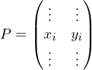
By writing the points as a matrix

We can write the smoothing operator as a matrix vector product

where is a sparse matrix with on the main diagonal and on the two minor diagonals.

is symmetric. Thus, it has an orthogonal basis of eigenvectors . We can represent in this basis:

where are suitable (two-dimensional) coefficients.

Applying to can now be written as



Thus, we can interpret smoothing as a scaling of the eigenvectors of .

TODO: Eigenfunctions of U and DFT

Filter Design
Our smoothing operator reduces mid and high frequencies of the mesh. Thus,

only contains the low frequencies of the input. By subtraction, we get the mid and high frequency parts:


We now apply our smoothing operator only to those mid and high frequencies:


Combining the low and smoothed high frequency terms gives:


Which is a smoothing operator which only dampens the mid and high frequencies.