Schwerpunktkolloquium: Basic Techniques, Geometry Processing, Global Illumination (116 Cards)
Name all OpenGL shader stages in the correct order. Which data is passed from one stage to the next?
Vertex Shader
(mandatory)
Executed for every vertex
Input: Attribute values as defined by vertex data
Output: Attribute values
Tessellation Control Shader
Executed for every primitive (triangle, line, patch)
Input: Attribute values
Output: Attribute values, requested degree of tessellation
Tessellation Evaluation Shader
Executed for every vertex of the tessellated primitive
Input: Attribute values
Output: Attribute values, requested degree of tessellation
Geometry Shader
Executed for every primitive (triangle, line, point), possibly generated by the tessellation, possibly with information about adjacent primitives
Input: Array of attribute values
Output: Arbitrary number of primitives, each with possibly different attribute values
Fragment Shader
(mandatory)
Executed for every fragment
Input: Possibly interpolated attribute values
Output: Fragment data which is written to frame buffers
(mandatory)
Executed for every vertex
Input: Attribute values as defined by vertex data
Output: Attribute values
Tessellation Control Shader
Executed for every primitive (triangle, line, patch)
Input: Attribute values
Output: Attribute values, requested degree of tessellation
Tessellation Evaluation Shader
Executed for every vertex of the tessellated primitive
Input: Attribute values
Output: Attribute values, requested degree of tessellation
Geometry Shader
Executed for every primitive (triangle, line, point), possibly generated by the tessellation, possibly with information about adjacent primitives
Input: Array of attribute values
Output: Arbitrary number of primitives, each with possibly different attribute values
Fragment Shader
(mandatory)
Executed for every fragment
Input: Possibly interpolated attribute values
Output: Fragment data which is written to frame buffers
How many neighbors does each Voronoi cell have in a planar Voronoi diagram, on average?
In 2D, the Voronoi diagram is dual to the Delaunay triangulation. For each triangle mesh, we know that

i.e., each vertex is adjacent to 6 other vertices, on average. Since vertices in the Delaunay triangulation are dual to Voronoi cells, each Voronoi cell has 6 neighboring cells, on average.

i.e., each vertex is adjacent to 6 other vertices, on average. Since vertices in the Delaunay triangulation are dual to Voronoi cells, each Voronoi cell has 6 neighboring cells, on average.
Explain Parametrization-Based Quad Meshing (Mixed Integer Quadrangulation)
Input: Mesh of triangles  . For some triangles, we have a confident estimate of the local min / max curvature directions (e.g. computed using the Shape Operator) given by an angle
  relative to some reference edge
  .
.
Smooth Cross Field
We propagate a smooth cross field over the entire surface. For each edge we can define a smoothness energy

where and
and  are the cross field directions given as an angle with the reference edges
  and
and  , respectively.
  denotes the angle between the two reference edges.
 is an integer variable that allows
  rotations of the cross fields.
For the entire mesh, we construct the system

We solve this system for the real variables and the integer variables
  . For those triangles where an input cross field direction is known, we fix the value:
  .
.
Parametrization
For each triangle corner in the mesh, compute coordinates such that for each triangle,

becomes small. Globally:

In order to obtain a disk topology for parametrization, the surface needs to be cut open. As an additional constraint, we thus introduce the requirement, that the parametrization should be consistent across boundary edges. That means that the transformation of parameters across an edge should be a grid automorphism.
Specifically, given a boundary edge between two triangles
  and
and  we constrain the
  coordinates at the opposite sides of the vertices
  to be equal up to grid automorphisms. That means:


The integer variable is known from the smooth cross field. For
  ,
,  , we need to find integer solutions.
In order to ensure that the resulting mesh will be a quad mesh, we snap singularities to integer positions.
We can introduce additional hard alignment constraints in order to snap feature edges to integer iso-lines. If an edge should be snapped to a
  -integer-iso-line, we constrain the values of
  for vertices of
  to be integer.
Solving Mixed-Integer Problems
In general: NP-Hard. We approximate a solution by relaxing the problem: Find a real-valued solution. Snap integer variables to nearest possible value, repeat.
 . For some triangles, we have a confident estimate of the local min / max curvature directions (e.g. computed using the Shape Operator) given by an angle
  relative to some reference edge
  .
.Smooth Cross Field
We propagate a smooth cross field over the entire surface. For each edge
 we can define a smoothness energy
where
 and
and  are the cross field directions given as an angle with the reference edges
  and
and  , respectively.
  denotes the angle between the two reference edges.
 is an integer variable that allows
  rotations of the cross fields.
For the entire mesh, we construct the system

We solve this system for the real variables
 and the integer variables
  . For those triangles where an input cross field direction is known, we fix the value:
  .
.Parametrization
For each triangle corner in the mesh, compute
 coordinates such that for each triangle,
becomes small. Globally:

In order to obtain a disk topology for parametrization, the surface needs to be cut open. As an additional constraint, we thus introduce the requirement, that the parametrization should be consistent across boundary edges. That means that the transformation of parameters across an edge should be a grid automorphism.
Specifically, given a boundary edge
 between two triangles
  and
and  we constrain the
  coordinates at the opposite sides of the vertices
  to be equal up to grid automorphisms. That means:

The integer variable
 is known from the smooth cross field. For
  ,
,  , we need to find integer solutions.
In order to ensure that the resulting mesh will be a quad mesh, we snap singularities to integer positions.
We can introduce additional hard alignment constraints in order to snap feature edges to integer iso-lines. If an edge
 should be snapped to a
  -integer-iso-line, we constrain the values of
  for vertices of
  to be integer.
Solving Mixed-Integer Problems
In general: NP-Hard. We approximate a solution by relaxing the problem: Find a real-valued solution. Snap integer variables to nearest possible value, repeat.
How can we classify surface curvature in the continuous case? What is a discrete approximation for triangle meshes?
If we have a parametric surface  , we can take its taylor expansion

We can now reparametrize such that
  lies in the origin and the plane
  is parallel to


Since this matrix is symmetric and real-valued, we can do an eigendecomposition:

From the eigenvalues and
and  , we can derive two characteristics for local curvature:
Mean Curvature:
Gaussian Curvature:
Which has the following interpretations:
 : Cap / Peak / Valley (elliptic)
 : Cylinder (parabolic)
 : Saddle (hyperbolic)
The eigenvectors corresponding to and
and  represent the respective curvature directions and are orthogonal.
Shape Operator
Approximates curvature for triangle meshes.
For each edge : atomic shape operator

where is the angle between the triangle normals
 .
.
Around a vertex, we compute the atomic shape operators of all edges in the vicinity

where measures the length of the portion of the edge
  inside
  .
.
From this, we can compute:
The eigenvector to the largest eigenvalue of points into the direction of minimum curvature.
The direction of maximum curvature is orthogonal to that and can be found by taking the cross product with the normal vector.
We cannot derive the exact curvature values and
and  , but it is

 , we can take its taylor expansion
We can now reparametrize
 such that
  lies in the origin and the plane
  is parallel to


Since this matrix is symmetric and real-valued, we can do an eigendecomposition:

From the eigenvalues
 and
and  , we can derive two characteristics for local curvature:
Mean Curvature:

Gaussian Curvature:

Which has the following interpretations:
 : Cap / Peak / Valley (elliptic)
 : Cylinder (parabolic)
 : Saddle (hyperbolic)
The eigenvectors corresponding to
 and
and  represent the respective curvature directions and are orthogonal.
Shape Operator
Approximates curvature for triangle meshes.
For each edge
 : atomic shape operator
where
 is the angle between the triangle normals
 .
.Around a vertex, we compute the atomic shape operators of all edges in the vicinity

where
 measures the length of the portion of the edge
  inside
  .
.From this, we can compute:
The eigenvector to the largest eigenvalue of
 points into the direction of minimum curvature.
The direction of maximum curvature is orthogonal to that and can be found by taking the cross product with the normal vector.
We cannot derive the exact curvature values
 and
and  , but it is
What is the goal of Subdivision techniques? Explain Subdivision using the Lane-Riesenfeld technique!
We interpret a sequence of points  as the control points of a B-Spline curve

Now, we want to describe the same curve with a higher number of control points.
We define two operators on the sequence

Doubling

Averaging

To determine the new vertex positions, we compute weighted positions based on even / odd rules.
Subdivision Operators
Linear (primal)

Quadratic Spline (dual)

Cubic Spline (primal)

TODO: Fix this explanation
Consider the B-Spline basis function .
.
It is a piecewise linear function between


We can write as an affine combination of the same function with parameter
  :
:

We can do this for uniform B-Spline basis functions in general:

where

 as the control points of a B-Spline curve
Now, we want to describe the same curve with a higher number of control points.
We define two operators on the sequence

Doubling

Averaging

To determine the new vertex positions, we compute weighted positions based on even / odd rules.
Subdivision Operators
Linear (primal)

Quadratic Spline (dual)

Cubic Spline (primal)

TODO: Fix this explanation
Consider the B-Spline basis function
 .
.It is a piecewise linear function between


We can write
 as an affine combination of the same function with parameter
  :
:
We can do this for uniform B-Spline basis functions in general:

where

Prove why creating a Delaunay Triangulation using edge flipping terminates using Seidel's Parabolic Map!
Lift every vertex onto a parabola:

A circle in the plane maps to an ellipsoid on the parabola. This ellipsoid lies in a plane. Every point on the ground which lies inside the circle lifts to a point below the plane. Every point on the ground which lies outside the circle lifts to a point above the plane.
Suppose have a non-Delaunay pair of triangles ,
,  in the plane, where
  lies in
  's circumcircle.
The lifted points lie in the same plane as the lifted ellipse of
  's circumcircle. Since
  lies inside the circle,
 lies below the plane of
  . Thus, the edge
  is reflex.
By flipping the edge to
to  , we replace the reflex edge
  by the convex edge
  .
.
Note that the four points form a tetrahedron. Before the flip, our triangulation corresponded to the upward-facing faces of the tetrahedron. After the flip, it corresponded to the downward-facing faces of the tetrahedron.
Thus, with each flip, we monotonically decrease the height of our triangulation on the paraboloid. Tetrahedral edges which lie on the upward-facing side are never considered again. Thus, the algorithm terminates eventually.

A circle in the plane maps to an ellipsoid on the parabola. This ellipsoid lies in a plane. Every point on the ground which lies inside the circle lifts to a point below the plane. Every point on the ground which lies outside the circle lifts to a point above the plane.
Suppose have a non-Delaunay pair of triangles
 ,
,  in the plane, where
  lies in
  's circumcircle.
The lifted points
 lie in the same plane as the lifted ellipse of
  's circumcircle. Since
  lies inside the circle,
 lies below the plane of
  . Thus, the edge
  is reflex.
By flipping the edge
 to
to  , we replace the reflex edge
  by the convex edge
  .
.Note that the four points
 form a tetrahedron. Before the flip, our triangulation corresponded to the upward-facing faces of the tetrahedron. After the flip, it corresponded to the downward-facing faces of the tetrahedron.
Thus, with each flip, we monotonically decrease the height of our triangulation on the paraboloid. Tetrahedral edges which lie on the upward-facing side are never considered again. Thus, the algorithm terminates eventually.
Explain the idea of Free-Form Modeling!
General idea: The user defines two regions on a mesh:
A support region which should be affected by the modeling.
A handle region inside the support region which the user can transform freely. The support region between the handle and the rest of the mesh should interpolate smoothly.
Solution: Fix all vertex positions except those of the support region.
For the support region vertices, solve

i.e. compute a smooth interpolating surface.
Problem: Smoothly interpolated surface loses detail.
Detail Preservation
Input mesh .
.
Fix vertex positions in the handle and the non-support regions and compute smooth surface .
.
Compute detail offset mesh .
.
Let the user transform the handle region and compute a new smoothed mesh .
.
Re-add the detail information:
 .
.
For rotations: Store normal offsets instead of absolute position offsets.
A support region which should be affected by the modeling.
A handle region inside the support region which the user can transform freely. The support region between the handle and the rest of the mesh should interpolate smoothly.
Solution: Fix all vertex positions except those of the support region.
For the support region vertices, solve

i.e. compute a smooth interpolating surface.
Problem: Smoothly interpolated surface loses detail.
Detail Preservation
Input mesh
 .
.Fix vertex positions in the handle and the non-support regions and compute smooth surface
 .
.Compute detail offset mesh
 .
.Let the user transform the handle region and compute a new smoothed mesh
 .
.Re-add the detail information:
 .
.For rotations: Store normal offsets instead of absolute position offsets.
Explain the idea of Laplace Reconstruction / Laplace Editing!
The global shape of a mesh is encoded in its positions  .
.
The local shape of a mesh is encoded in its Laplace vectors .
.
Given all Laplace vectors of a mesh, we can reconstruct a global shape
  from the local shape:

We need to fix one intial vertex position and solve for the remaining variables
  .
.
We can also use this as an editing metaphor by letting the user prescribe desired positions for certain vertices
  . Incorporating this into the minimization formula gives

Additionally, we need to allow rotations of the detail vectors:

 .
.The local shape of a mesh is encoded in its Laplace vectors
 .
.Given all Laplace vectors
 of a mesh, we can reconstruct a global shape
  from the local shape:
We need to fix one intial vertex position
 and solve for the remaining variables
  .
.We can also use this as an editing metaphor by letting the user prescribe desired positions
 for certain vertices
  . Incorporating this into the minimization formula gives
Additionally, we need to allow rotations of the detail vectors:

Explain the GIST descriptor!
Describes the spatial color distribution in an image. Robust to small camera movements.
Store the averaged intensity values. Per color channel: values per image.
- Compute
 blurred versions of the input image, e.g. by convolutions with Gaussian kernels of increasing size.
 - For each blurred image, compute
 convolutions with gradient filters of different directions.
 - Partition each gradient image into
 sectors and compute an average intensity value for each sector.
Store the averaged intensity values. Per color channel:
 values per image.
How are Light Fields parametrized? How can we generate such a parametrization from a set of input images?
Two-Plane Parametrization
Assuming the scene is contained between two parallel planes, the camera plane and the object plane, we can parametrize each ray by a point on the camera plane and a point
  on the object plane. The radiance along that ray is given by

Light Field Generation
1. Re-projection / Rectification of input images
2. Re-binning to produce uniform sampling on camera and object plane
Rectification
Each input image was taken at a camera position with a projection matrix
  projecting a point
  to a point
  on the camera plane.
 is a transformation from 3D homogenous coordinates to 2D homogenous coordinates. Thus,

We want to project from the same camera position
  onto a different projection plane given by another projection matrix
  which has the same layout as
Since the coordinate of
  is 1, we can write


We now multiply the first equation by on both sides:


Thus, we can transform projected points from the input image into projected points of the output image
  by applying the
  homography

Re-Binning
When rectifying several images from different viewpoints, we obtain an uneven sampling on the camera / object plane. We get a uniform sampling by discretizing the light field and applying the Pull-Push algorithm to provide a color value for every pixel.
Pull-Push algorithm
Explained in 2D here. For Light Fields, we need to do this in 4D. Given: 2D grid of cells and unevenly distributed color samples which are assigned to cells
  .
.
For each cell, store a color value and a weight
  .
.
Initialization
For each cell, compute an average color and an initial weight


Pull
Average colors and sum weights onto higher levels


Push
For each cell on the base level, walk up the hierarchy until a cell with weight > 0 is found. Use the color of that cell.
Assuming the scene is contained between two parallel planes, the camera plane and the object plane, we can parametrize each ray by a point
 on the camera plane and a point
  on the object plane. The radiance along that ray is given by
Light Field Generation
1. Re-projection / Rectification of input images
2. Re-binning to produce uniform sampling on camera and object plane
Rectification
Each input image was taken at a camera position
 with a projection matrix
  projecting a point
  to a point
  on the camera plane.
 is a transformation from 3D homogenous coordinates to 2D homogenous coordinates. Thus,
We want to project
 from the same camera position
  onto a different projection plane given by another projection matrix
  which has the same layout as
Since the
 coordinate of
  is 1, we can write

We now multiply the first equation by
 on both sides:


Thus, we can transform projected points
 from the input image into projected points of the output image
  by applying the
  homography
Re-Binning
When rectifying several images from different viewpoints, we obtain an uneven sampling on the camera / object plane. We get a uniform sampling by discretizing the light field and applying the Pull-Push algorithm to provide a color value for every pixel.
Pull-Push algorithm
Explained in 2D here. For Light Fields, we need to do this in 4D. Given: 2D grid of cells and unevenly distributed color samples
 which are assigned to cells
  .
.For each cell, store a color value
 and a weight
  .
.Initialization
For each cell, compute an average color and an initial weight


Pull
Average colors and sum weights onto higher levels


Push
For each cell on the base level, walk up the hierarchy until a cell with weight > 0 is found. Use the color of that cell.
How are Light Fields rendered? How can we do this on the GPU?
First, consider bi-linear interpolation. In order to determine the color at a position  lying between four grid samples. Each grid sample at a position
  has an influence of

on .
.
Given: Light Field
Let be the coordinates of the four pixels around
  on the camera plane and
  the coordinates of the four pixels around
  on the object plane.
For each , we compute an interpolated color value
  from the four neighboring samples
  on the object plane based on the position
  .
.
Then, we compute a interpolated color value from the , based on the position
  .
.
Since we do a linear interpolation twice, this is called quad-linear interpolation.
GPU Implementation
Obtaining coordinates for every pixel
Draw two quads: One for the object plane, one for the camera plane. As a texture, use a smooth color gradient from lower left to
  upper right. The rasterized colors are the
  coordinates for every pixel.
Bi-Linear Interpolation on the Object Plane
We get this for free through texture interpolation: For each camera plane pixel, render one quad. As texture coordinates for the quad, use the respective coordinates at that position.
Quad-Linear Interpolation
Instead of rendering one quad per camera plane pixel, render four quads surrounding the pixel with alpha blending and fade out the contribution towards the outer edges.
 lying between four grid samples. Each grid sample at a position
  has an influence of
on
 .
.Given: Light Field

Let
 be the coordinates of the four pixels around
  on the camera plane and
  the coordinates of the four pixels around
  on the object plane.
For each
 , we compute an interpolated color value
  from the four neighboring samples
  on the object plane based on the position
  .
.Then, we compute a interpolated color value from the
 , based on the position
  .
.Since we do a linear interpolation twice, this is called quad-linear interpolation.
GPU Implementation
Obtaining
 coordinates for every pixel
Draw two quads: One for the object plane, one for the camera plane. As a texture, use a smooth color gradient from
 lower left to
  upper right. The rasterized colors are the
  coordinates for every pixel.
Bi-Linear Interpolation on the Object Plane
We get this for free through texture interpolation: For each camera plane pixel, render one quad. As texture coordinates for the quad, use the respective
 coordinates at that position.
Quad-Linear Interpolation
Instead of rendering one quad per camera plane pixel, render four quads surrounding the pixel with alpha blending and fade out the contribution towards the outer edges.
What is a Lumigraph? How must we update our object plane coordinates for Lumigraph rendering?
Lumigraph
Light Field + depth information. For a ray , we can compute a depth value
  telling at which depth between the camera and object plane the ray intersects the geometry.
This allows us to do more accurate interpolation by offsetting sample coordinates on the object plane.
Coordinate Offset
Let's consider the 2D case where a ray is only parametrized by and
and  .
.
For each grid point around
  , we would compute a interpolated color for
  . However, if the ray through
  and
and  intersects a surface at a distance of
  to the camera plane, we could find a better ray from
  to another point
  which intersects the geometry at the same point.
This is easily found by comparing similar triangles:


Light Field + depth information. For a ray
 , we can compute a depth value
  telling at which depth between the camera and object plane the ray intersects the geometry.
This allows us to do more accurate interpolation by offsetting sample coordinates on the object plane.
Coordinate Offset
Let's consider the 2D case where a ray is only parametrized by
 and
and  .
.For each grid point
 around
  , we would compute a interpolated color for
  . However, if the ray through
  and
and  intersects a surface at a distance of
  to the camera plane, we could find a better ray from
  to another point
  which intersects the geometry at the same point.
This is easily found by comparing similar triangles:


What is an Unstructured Lumigraph? How does Unstructured Lumigraph rendering work? How can we do this in hardware?
Input Data
Unstructured set of photos (with calibration information and camera positions)
Proxy Geometry
Requirements
Render interpolated views of the scene
Rendering
For each pixel of the output image, compute a blending of the input images. First, compute view ray by intersecting with proxy geometry, then find k-best input images.
For each input image , compute the angle difference
  at the intersection point.
We denote by the angle difference of the k-best camera. Now, we can compute the color contribution of each image as

and normalizing

To improve consistency, we can emphasize weights where the angle is very small, e.g.:

Hardware Implementation
Tessellate screen with a triangle grid. Insert into this grid:
Compute blending weights for triangle vertices. Render each triangle several times (at least , at most
  times) with the appropriate textures and additive blending.
Unstructured set of photos (with calibration information and camera positions)
Proxy Geometry
Requirements
Render interpolated views of the scene
- in real time
- with no pre-processing or re-sampling of the input images
- with smooth interpolation as the camera moves through the scene
- consistent (reproduce source image if desired viewpoint matches)
Rendering
For each pixel of the output image, compute a blending of the input images. First, compute view ray by intersecting with proxy geometry, then find k-best input images.
For each input image
 , compute the angle difference
  at the intersection point.
We denote by
 the angle difference of the k-best camera. Now, we can compute the color contribution of each image as
and normalizing

To improve consistency, we can emphasize weights where the angle is very small, e.g.:

Hardware Implementation
Tessellate screen with a triangle grid. Insert into this grid:
- Edges of the proxy geometry (here are discontinuities)
- Epipolar points of the cameras (we want the image to be consistent there)
Compute blending weights for triangle vertices. Render each triangle several times (at least
 , at most
  times) with the appropriate textures and additive blending.
What are Layered Depth Images? How to render them with correct occlusion?
Input: Set of images with colors and depth information.
Layered Depth Image: All of these input images combined into one image (from a new viewpoint), where along each viewing ray there may be several pixels with different depths and colors.
We can render an LDI by splatting all points. Points are transformed by the camera matrix:

 can be decomposed into 4 row vectors:
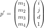
If we know a transformed point , new points in the vicinity can be computed incrementally:

Correct occlusion can be ensured by projecting the camera position into the LDI. This point splits the LDI into 4 quadrants which are rendered row-wise outside-inwards towards the epipolar point.
Layered Depth Image: All of these input images combined into one image (from a new viewpoint), where along each viewing ray there may be several pixels with different depths and colors.
We can render an LDI by splatting all points. Points are transformed by the camera matrix:

 can be decomposed into 4 row vectors:
If we know a transformed point
 , new points in the vicinity can be computed incrementally:
Correct occlusion can be ensured by projecting the camera position into the LDI. This point splits the LDI into 4 quadrants which are rendered row-wise outside-inwards towards the epipolar point.
What are Image-Based Visual Hulls?
Input: Set of images where on each image, there is an identifiable silhouette of the shown object. Each camera spans a generalized cone through the silhouette. The intersection of all these cones approximates the shape of the object.
Goal: For a new viewpoint, find out where the view ray intersects the approximated shape of the object.
In each source image, the projection of the view ray for one pixel in the target image is a line. We want to find the intersection points of this line with the silhouette. Thus, we discretize the silhouette into line segments and test for intersections: complexity per source image.
Note that if the camera position is fixed, the projected view rays in the source images are a pencil of lines through the camera epipolar point. Every time the camera position changes, perform a binning of the polygon edges into sectors. This reduces the intersection complexity from to
to  .
.
Goal: For a new viewpoint, find out where the view ray intersects the approximated shape of the object.
In each source image, the projection of the view ray for one pixel in the target image is a line. We want to find the intersection points of this line with the silhouette. Thus, we discretize the silhouette into line segments and test for intersections:
 complexity per source image.
Note that if the camera position is fixed, the projected view rays in the source images are a pencil of lines through the camera epipolar point. Every time the camera position changes, perform a binning of the polygon edges into sectors. This reduces the intersection complexity from
 to
to  .
.What is Image Retargeting? How can we do it?
Image Retargeting
Change of image dimensions without stretching / cropping in regions where there is interesting content.
We first need a salience measure that tells us which areas of an image are interesting or important and should be preserved. Generally involves some kind of gradient filter / Laplace filter / sobel filter, or similar.
Seam Carving
Assuming we want to reduce the width of the image.
Find continuous, monotonic path from top to bottom through the image (seam) which has minimal total salience. Remove this seam.
Repeat until target width reached.
We denote by the lowest cost of a seam starting at pixel
  and running to the bottom of the image (
 ).
).
Of course, for the bottom line pixels, this is just the local salience value:

For all other pixels, the minimum cost is computed as

A solution to this can be computed using Dynamic Programming.
An alternative solution approach is to formulate the seam search as a min-cost graph cut problem.
Change of image dimensions without stretching / cropping in regions where there is interesting content.
We first need a salience measure that tells us which areas of an image are interesting or important and should be preserved. Generally involves some kind of gradient filter / Laplace filter / sobel filter, or similar.
Seam Carving
Assuming we want to reduce the width of the image.
Find continuous, monotonic path from top to bottom through the image (seam) which has minimal total salience. Remove this seam.
Repeat until target width reached.
We denote by
 the lowest cost of a seam starting at pixel
  and running to the bottom of the image (
 ).
).Of course, for the bottom line pixels, this is just the local salience value:

For all other pixels, the minimum cost is computed as

A solution to this can be computed using Dynamic Programming.
An alternative solution approach is to formulate the seam search as a min-cost graph cut problem.
Explain Image Completion!
Problem
Input image with some area (the hole) which should be filled with data from the rest of the image.
Idea
Repeatedly shrink the hole by:
Selecting an area which overlaps both the hole and a part of the image around it.
Finding a region (fragment) in the image which is similar to .
.
Copying over the pixels from the fragment into the hole.
Finding
We search for an optimal pixel offset such that


The first term is constant w.r.t. .
.
The third term can be computed in with some precomputations.
What remains is the middle term which corresponds to a convolution. We can compute this by transforming both the input image as well as the region into the frequency domain and then doing the multiplication there. We then transform back to the pixel domain and find the maximum intensity pixel.
Compositing
After we have found the best source fragment, we compute an ideal seam for the fragment we copy over. This can be computed by a min-flow graph cut.
Color Correction
Additionally, we adjust the color of the copied-over pixels such that they match the hole boundary. We do this by prescribing that the color corrected pixels should have the same color gradients as the source pixels

while on the boundary, there should be no color difference

By applying the divergence on both sides, we turn this into a Poisson Equation


Perspective Correction
Sometimes, we want to reconstruct pixels from parts of the image which are viewed at an angle. Let the user define piecewise homographies by painting in the vertices of square patches. Flatten the image by applying the homographies and use this flattened image for the image completion.
Input image with some area (the hole) which should be filled with data from the rest of the image.
Idea
Repeatedly shrink the hole by:
Selecting an area which overlaps both the hole and a part
 of the image around it.
Finding a region (fragment) in the image which is similar to
 .
.Copying over the pixels from the fragment into the hole.
Finding
We search for an optimal pixel offset
 such that

The first term is constant w.r.t.
 .
.The third term can be computed in
 with some precomputations.
What remains is the middle term which corresponds to a convolution. We can compute this by transforming both the input image as well as the region
 into the frequency domain and then doing the multiplication there. We then transform back to the pixel domain and find the maximum intensity pixel.
Compositing
After we have found the best source fragment, we compute an ideal seam for the fragment we copy over. This can be computed by a min-flow graph cut.
Color Correction
Additionally, we adjust the color of the copied-over pixels such that they match the hole boundary. We do this by prescribing that the color corrected pixels
 should have the same color gradients as the source pixels

while on the boundary, there should be no color difference

By applying the divergence on both sides, we turn this into a Poisson Equation


Perspective Correction
Sometimes, we want to reconstruct pixels from parts of the image which are viewed at an angle. Let the user define piecewise homographies by painting in the vertices of square patches. Flatten the image by applying the homographies and use this flattened image for the image completion.
Give the smoothing operator for 3D meshes! Which weights can we use for this?
Smoothing Operator

Uniform Weights

Move vertices into center of gravity of its 1-ring neighbors. Performs normal and tangential smoothing. Leads to a regular distribution of vertices.
Cotangent Weights

Denoting the area of the 1-ring around by
by  , cotangent weights move
  into the direction of
  . Since in a planar configuration, moving
  does not change
  ,
,  is normal to the mesh. Thus, cotangent weights have linear precision. Cotangent weights mostly do normal smoothing. They can become negative for very long triangles. However, if the mesh is Delaunay, Cotangent weights are positive.
Mean Value Weights

where and
and  are the angles between the edge
  and the edges to the previous and next 1-ring neighbor, respectively. MVW have linear precision, they are always positive, but they are non-symmetric:
 , in general

Uniform Weights

Move vertices into center of gravity of its 1-ring neighbors. Performs normal and tangential smoothing. Leads to a regular distribution of vertices.
Cotangent Weights

Denoting the area of the 1-ring around
 by
by  , cotangent weights move
  into the direction of
  . Since in a planar configuration, moving
  does not change
  ,
,  is normal to the mesh. Thus, cotangent weights have linear precision. Cotangent weights mostly do normal smoothing. They can become negative for very long triangles. However, if the mesh is Delaunay, Cotangent weights are positive.
Mean Value Weights

where
 and
and  are the angles between the edge
  and the edges to the previous and next 1-ring neighbor, respectively. MVW have linear precision, they are always positive, but they are non-symmetric:
 , in general
Give a physical interpretation of smoothing operators!
If we iterate the smoothing operator

until convergence, the will go to zero:

We know that approximates the Laplace of a function that interpolates the
  . Thus

The physical interpretation of is an area-minimizing membrane surface, comparable to the surface of a soap film suspended inside a wire loop.
By constraining higher-order derivatives of , we can model other surfaces such as a thin plate:

which gives

and produces a surface which minimizes curvature.

until convergence, the
 will go to zero:
We know that
 approximates the Laplace of a function that interpolates the
  . Thus
The physical interpretation of
 is an area-minimizing membrane surface, comparable to the surface of a soap film suspended inside a wire loop.
By constraining higher-order derivatives of
 , we can model other surfaces such as a thin plate:
which gives

and produces a surface which minimizes curvature.
How to prevent a mesh from shrinking too much when applying smoothing?
Error Control
Constrain the positions of the vertices such that they can only move by a certain extent from their original position.
 -Balls
A vertex must not move by more than
  from its original position
  .
.
If leaves its
  ball after a smoothing iteration, it is projected back onto the closest point inside the ball:

Error Slabs
The movement of a vertex is constrained to its original tangent plane. Its position may not deviate from the tangent plane by more than
  . If it does, it is projected back:

Constrain the positions of the vertices such that they can only move by a certain extent from their original position.
 -Balls
A vertex
 must not move by more than
  from its original position
  .
.If
 leaves its
  ball after a smoothing iteration, it is projected back onto the closest point inside the ball:
Error Slabs
The movement of a vertex
 is constrained to its original tangent plane. Its position may not deviate from the tangent plane by more than
  . If it does, it is projected back:
Explain the Incremental Decimation algorithm!
Algorithm Overview
for each local operator:
evaluate quality decrease
enqueue (quality decrease, op) into priority queue
repeat:
pop best operator from queue
apply
update queue
until target complexity reached or error too large
Operators
Error Metrics
Local Error Metrics: Plane distance, Volume change
Global Error Metrics: Hausdorff distance, Simplification Envelopes, Error Quadrics
Error Quadrics are particularly suitable because they can be evaluated locally: On the initial mesh, compute error quadrics for every vertex from its incident triangle planes. When two vertices are merged, the error quadrics stored in the original vertices are added. Note: Not 100% correct since some planes are added twice.
Fairness Criteria
To ensure a certain mesh quality, we can forbid some operators:
for each local operator:
evaluate quality decrease
enqueue (quality decrease, op) into priority queue
repeat:
pop best operator from queue
apply
update queue
until target complexity reached or error too large
Operators
- Vertex Removal: Remove center vertex from a 1-ring and re-triangulate. Topological operator. Degrees of freedom: Triangulation.
- Edge Collapse: Merge the two end vertices of one edge into one. Topological / geometrical operator. Degrees of freedom: Vertex position.
- Halfedge Collapse: Merge the start vertex and the end vertex of one edge. New position is the position of the end vertex. Topological operator. Degrees of freedom: None (which is preferable).
Error Metrics
Local Error Metrics: Plane distance, Volume change
Global Error Metrics: Hausdorff distance, Simplification Envelopes, Error Quadrics
Error Quadrics are particularly suitable because they can be evaluated locally: On the initial mesh, compute error quadrics for every vertex from its incident triangle planes. When two vertices are merged, the error quadrics stored in the original vertices are added. Note: Not 100% correct since some planes are added twice.
Fairness Criteria
To ensure a certain mesh quality, we can forbid some operators:
- Triangle Shape: Forbid operators which would produce triangles with too small interior angles
- Valence Balance: Forbid operators which would produce a triangulation where the valence of a vertex becomes very small or very large
- Normal Approximation
- Texture Distortion
How are Progressive Meshes generated, stored and reconstructed? How can we do Selective Refinement?
Original mesh: 
Incremental Decimation applies a series of decimation operators:

By reversing these operators, we can reconstruct from the decimated mesh

In order to make a Halfedge Collapse operator reversible, we need to store:
Thus, each operator is stored as

Selective Refinement
If we want to undo an operator

the problem might be that one of the opposite vertices or
or  does not exist:
In order to solve this problem, we store the refined mesh as a binary forest where the leaf nodes are the unrefined vertices and each inner node corresponds to a decimation operator.
During decimation, we remember from which original vertices our mesh started out. Initially, we store at every triangle corner a pointer to the incident vertex. As we decimate the mesh, these triangle corner labels remain intact. When we store an operator, instead of storing ,
,  as the vertices in the decimated mesh, we store the values stored in the respective triangle corners.
If we want to refine at a vertex , we find the two opposite vertices
  ,
,  in the currently refined mesh by walking up the binary forest of operators until we find vertices that have already been instantiated.

Incremental Decimation applies a series of decimation operators:

By reversing these operators, we can reconstruct
 from the decimated mesh

In order to make a Halfedge Collapse operator
 reversible, we need to store:
- Position of the source vertex which was collapsed:

- A pointer to the target vertex towards which
 was collapsed:
- Pointers to the two boundary vertices which were adjacent to both
 and
and  before the collapse:
Thus, each operator is stored as

Selective Refinement
If we want to undo an operator

the problem might be that one of the opposite vertices
 or
or  does not exist:
-
 /
/  might not exist yet if it is still not expanded
 -
 /
/  might not exist anymore if it has previously been split
In order to solve this problem, we store the refined mesh as a binary forest where the leaf nodes are the unrefined vertices and each inner node corresponds to a decimation operator.
During decimation, we remember from which original vertices our mesh started out. Initially, we store at every triangle corner a pointer to the incident vertex. As we decimate the mesh, these triangle corner labels remain intact. When we store an operator, instead of storing
 ,
,  as the vertices in the decimated mesh, we store the values stored in the respective triangle corners.
If we want to refine at a vertex
 , we find the two opposite vertices
  ,
,  in the currently refined mesh by walking up the binary forest of operators until we find vertices that have already been instantiated.
Give a smoothing operator for a curve of vertices in 2D space! What analytical meaning does this operator have? How can we design a better smoothing operator?
Given: Line of vertices 
An intuitive smoothing operator is

or

with

Assuming the points are generated by an arc-length parametrized function


we can approximate the first derivative by divided differences:


And the second derivative by again taking divided differences:


Thus, the smoothing operator approximates the second derivative of the curve.
By writing the points as a matrix
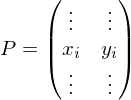
We can write the smoothing operator as a matrix vector product

where is a sparse matrix with
  on the main diagonal and
  on the two minor diagonals.
 is symmetric. Thus, it has an orthogonal basis of eigenvectors
  . We can represent
  in this basis:

where are suitable (two-dimensional) coefficients.
Applying to
to  can now be written as


Thus, we can interpret smoothing as a scaling of the eigenvectors of .
.
TODO: Eigenfunctions of U and DFT
Filter Design
Our smoothing operator reduces mid and high frequencies of the mesh. Thus,

only contains the low frequencies of the input. By subtraction, we get the mid and high frequency parts:


We now apply our smoothing operator only to those mid and high frequencies:


Combining the low and smoothed high frequency terms gives:


Which is a smoothing operator which only dampens the mid and high frequencies.

An intuitive smoothing operator is

or

with

Assuming the points are generated by an arc-length parametrized function


we can approximate the first derivative by divided differences:


And the second derivative by again taking divided differences:


Thus, the smoothing operator approximates the second derivative of the curve.
By writing the points as a matrix

We can write the smoothing operator as a matrix vector product

where
 is a sparse matrix with
  on the main diagonal and
  on the two minor diagonals.
 is symmetric. Thus, it has an orthogonal basis of eigenvectors
  . We can represent
  in this basis:
where
 are suitable (two-dimensional) coefficients.
Applying
 to
to  can now be written as


Thus, we can interpret smoothing as a scaling of the eigenvectors of
 .
.TODO: Eigenfunctions of U and DFT
Filter Design
Our smoothing operator reduces mid and high frequencies of the mesh. Thus,

only contains the low frequencies of the input. By subtraction, we get the mid and high frequency parts:


We now apply our smoothing operator only to those mid and high frequencies:


Combining the low and smoothed high frequency terms gives:


Which is a smoothing operator which only dampens the mid and high frequencies.
What is Mesh Decimation? Which algorithms did we look at and what kind of control do they provide?
In Mesh Decimation, given an input mesh, we try to find another mesh which looks similar but consists of fewer vertices. We would like to bound the approximation error of the decimated mesh. Also, we want to be able to prescribe a target complexity by giving the desired amount of vertices.
| Algorithm | Approximation Error | Target Complexity |
| Vertex Clustering | yes | |
| Incremental Decimation | yes | yes |
| Remeshing | yes |
Explain how to use Error Quadrics to compute the closest point to a set of planes!
We can represent a plane by

if
and a point by

Then, the distance from to the plane is given by

Given a set of planes , we want to find a point
  which minimizes the squared distances to all planes:


The matrices are called fundamental error quadrics and are computed as

From this definition, we see that the error quadrics of two sets of planes ,
,  can simply be merged into one error quadric by adding them:

Solution Approach 1
In order to find a minimum solution for , we can find the eigenvector to the smallest eigenvalue of
  .
.
Solution Approach 2
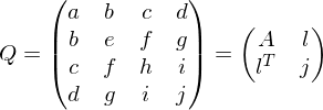
By computing

we obtain the linear system


Which is easier to solve than computing the eigenvectors and eigenvalues of .
.

if

and a point by

Then, the distance from
 to the plane is given by
Given a set of planes
 , we want to find a point
  which minimizes the squared distances to all planes:


The matrices
 are called fundamental error quadrics and are computed as
From this definition, we see that the error quadrics of two sets of planes
 ,
,  can simply be merged into one error quadric by adding them:
Solution Approach 1
In order to find a minimum solution for
 , we can find the eigenvector to the smallest eigenvalue of
  .
.Solution Approach 2

By computing

we obtain the linear system


Which is easier to solve than computing the eigenvectors and eigenvalues of
 .
.Explain Mesh Decimation using Vertex Clustering! What are the advantages / disadvantages of the method? How can Vertex Clustering be implemented out-of-core?
Idea
1. Impose a voxel grid on the input mesh.
2. For each cell containing vertices, compute a cell representative.
3. Create a new mesh which only has cell representatives as vertices. Three cell representatives are connected with a triangle if there was a triangle in the original mesh wich had one vertex in each of the three cells.
Quality Control
The approximation error is bounded by the voxel resolution : Vertices are shifted by at most
  .
.
Cell Representative
Advantages
Out-of-core implementation possible
Works on arbitrary geometry (no manifold required)
Disadvantages
Output mesh not guaranteed to be manifold
Loss of detail due to uniform sampling
Out-Of-Core Implementation
Required storage: One error quadric for every cell. Connectivity information (list of cells which need to be connected).
Processing: Read one triangle at a time. If the vertices fall into three different cells, keep a record on the connectivity list. Add the fundamental error quadric of the triangle to the cells of the vertices. After all triangles have been read, compute cell representatives and connect them.
1. Impose a voxel grid on the input mesh.
2. For each cell containing vertices, compute a cell representative.
3. Create a new mesh which only has cell representatives as vertices. Three cell representatives are connected with a triangle if there was a triangle in the original mesh wich had one vertex in each of the three cells.
Quality Control
The approximation error is bounded by the voxel resolution
 : Vertices are shifted by at most
  .
.Cell Representative
- Cell Center: Requires no computation but leads to bad approximation error and produces stair artifacts.
- Center of Gravity: Slightly better approximation. Introduces low-pass filter.
- Median: i.e. closest point to center of gravity. Less pronounced low pass.
- Error Quadric: Find least-squares closest point to all triangle planes in the cell. Produces best sampling of sharp features.
Advantages
Out-of-core implementation possible
Works on arbitrary geometry (no manifold required)
Disadvantages
Output mesh not guaranteed to be manifold
Loss of detail due to uniform sampling
Out-Of-Core Implementation
Required storage: One error quadric for every cell. Connectivity information (list of cells which need to be connected).
Processing: Read one triangle at a time. If the vertices fall into three different cells, keep a record on the connectivity list. Add the fundamental error quadric of the triangle to the cells of the vertices. After all triangles have been read, compute cell representatives and connect them.
How are rotations represented by quaternions?
Quaternions are hypercomplex numbers

where

We define the conjugate

the dot product

and the norm

By associating quaternions with vectors in , the product of two quaternions
  ,
,  can be written as a matrix-vector product


From the structure of these matrices, we can show the dot product equivalence


We can embed points into
into  as follows:

It can be shown that unit quaternions represent rotations. In particular, given a rotation axis where
where  and an angle
  , we can construct

Then, this rotation can be computed as


Note that and
and  represent the same rotation since both the rotation axis as the magnitude are inverted.
It turns out that


where

We define the conjugate

the dot product

and the norm

By associating quaternions with vectors in
 , the product of two quaternions
  ,
,  can be written as a matrix-vector product

From the structure of these matrices, we can show the dot product equivalence


We can embed points
 into
into  as follows:
It can be shown that unit quaternions represent rotations. In particular, given a rotation axis
 where
where  and an angle
  , we can construct
Then, this rotation can be computed as


Note that
 and
and  represent the same rotation since both the rotation axis as the magnitude are inverted.
It turns out that

How to register two patches obtained by a laser scanner using the Iterative Closest Point algorithm?
Assumption: Scanned patches have identical scale.
Goal: Find a rigid transformation (rotation and translation) for one of the patches to align it with the other.
Algorithm Overview
1. Initial alignment: Provided by the user
2. Matching: Find corresponding points in the two patches
3. Registration: Compute optimal translation and rotation
4. Repeat from step 2 until convergence.
Matching
Matching Strategy: Nearest Neighbor
For every vertex in patch
  , select the nearest neighbor vertex
  from patch
  .
.
Filtering: Remove those matchings where one vertex is a boundary vertex (since boundary vertices match to many points). Remove matchings with a high distance. Remove matchings with a high normal deviation.
Matching Strategy: Normal Piercing
From each vertex in patch
  , shoot a ray into normal direction. If this ray intersects with
  in point
  , add the correspondence
  .
.
Registration
Given a list of corresponding vertices
we want to find a transformation such that

Finding the translational part just amounts to shifting the center of gravity of the
  into that of the
  by adding an offset


We just assume this translational registration has already taken place and just focus on the rotational alignment:


The first and last term are independent of


Problem: Finding a solution for the rotation matrix requires finding 9 unknowns (of which 6 need to be constrained). Solution: Formulate the rotation as a quaternion (gives 4 unknowns with 1 additional constraint).


 is a symmetric matrix. To compute a solution for
  , find the eigenvector to the largest eigenvalue. Normalize to obtain a rotation.
Goal: Find a rigid transformation (rotation and translation) for one of the patches to align it with the other.
Algorithm Overview
1. Initial alignment: Provided by the user
2. Matching: Find corresponding points in the two patches
3. Registration: Compute optimal translation and rotation
4. Repeat from step 2 until convergence.
Matching
Matching Strategy: Nearest Neighbor
For every vertex
 in patch
  , select the nearest neighbor vertex
  from patch
  .
.Filtering: Remove those matchings where one vertex is a boundary vertex (since boundary vertices match to many points). Remove matchings with a high distance. Remove matchings with a high normal deviation.
Matching Strategy: Normal Piercing
From each vertex
 in patch
  , shoot a ray into normal direction. If this ray intersects with
  in point
  , add the correspondence
  .
.Registration
Given a list of corresponding vertices

we want to find a transformation
 such that
Finding the translational part
 just amounts to shifting the center of gravity of the
  into that of the
  by adding an offset

We just assume this translational registration has already taken place and just focus on the rotational alignment:


The first and last term are independent of


Problem: Finding a solution for the rotation matrix
 requires finding 9 unknowns (of which 6 need to be constrained). Solution: Formulate the rotation as a quaternion (gives 4 unknowns with 1 additional constraint).


 is a symmetric matrix. To compute a solution for
  , find the eigenvector to the largest eigenvalue. Normalize to obtain a rotation.
After two mesh patches have been registered (e.g. using ICP), how are they integrated? Explain the two main approaches!
Given: Two aligned patches  and
and  with some overlap.
Zippering
Remove overlap: Shoot rays from vertices of in normal direction. Remove triangles of
  which are hit. Then, do the same thing the other way around.
Merge: Walk along the two new patch boundaries and insert triangles to connect them.
Problem: This approach throws away a significant amount of detail information near the overlap region.
Stitching
Move the boundary vertices of patch along their normals so they lie on
  .
.
Insert boundary vertices of patch into
into  by splitting triangles.
Insert the boundary edges of patch into
into  by splitting edges.
Remove the overlapping part of patch .
.
 and
and  with some overlap.
Zippering
Remove overlap: Shoot rays from vertices of
 in normal direction. Remove triangles of
  which are hit. Then, do the same thing the other way around.
Merge: Walk along the two new patch boundaries and insert triangles to connect them.
Problem: This approach throws away a significant amount of detail information near the overlap region.
Stitching
Move the boundary vertices of patch
 along their normals so they lie on
  .
.Insert boundary vertices of patch
 into
into  by splitting triangles.
Insert the boundary edges of patch
 into
into  by splitting edges.
Remove the overlapping part of patch
 .
.Name two approaches for Mesh Repair! What are their advantages and disadvantages?
| Volumetric Mesh Repair | Surface-Based Mesh Repair |
| resulting mesh is guaranteed to be watertight and manifold | no guarantee on output quality |
| voxelization: may suffer from aliasing / sampling artifacts or loss of precision | structure-preserving: only modifies input mesh where necessary |
Explain Volumetric Mesh Repair!
Input: "Triangle Soup"  : Collection of surface parts which may contain gaps, intersections or other problems
Output: Watertight two-manifold mesh
Parameters:
 : approximation tolerance
 : maximum hole / gap size
Requirements:

"every point on the original mesh has a distance of at most to a point on the reconstructed mesh"
also: but only if the closest point on
  is not a boundary point

"every point on the reconstructed mesh has a distance of at most to a point on the original mesh"
Algorithm
Insert all mesh faces into a voxel grid.
Grow -blobs from all boundary edges.
Flood fill the exterior.
Erode the -blobs from outside.
Reconstruct the mesh using Marching Cubes.
 : Collection of surface parts which may contain gaps, intersections or other problems
Output: Watertight two-manifold mesh

Parameters:
 : approximation tolerance
 : maximum hole / gap size
Requirements:

"every point on the original mesh has a distance of at most
 to a point on the reconstructed mesh"
also:
 but only if the closest point on
  is not a boundary point
"every point on the reconstructed mesh has a distance of at most
 to a point on the original mesh"
Algorithm
Insert all mesh faces into a voxel grid.
Grow
 -blobs from all boundary edges.
Flood fill the exterior.
Erode the
 -blobs from outside.
Reconstruct the mesh using Marching Cubes.
Explain Surface-Based Hole Filling! What are some problems of this approach?
Input: Boundary loop consisting of vertices  .
.
Goal: Triangulation of the loop interior which minimizes some triangulation cost
  which is a combination of e.g.
which produces a hole filling with low area and low normal deviation.
We denote by the cost of the best triangulation for only the vertices
  .
.
Obviously:


Solve using dynamic programming.
Complexity: (Compute table for
  and
and  . For every entry, consider
  possible middle triangles)
Optional post-processing steps
Refine the triangulation of the hole.
Apply smoothing to the hole region.
Problems
Does not work for islands.
Does not consider self-intersections.
 .
.Goal: Triangulation
 of the loop interior which minimizes some triangulation cost
  which is a combination of e.g.
- the area of the triangles
- the maximum dihedral angle
which produces a hole filling with low area and low normal deviation.
We denote by
 the cost of the best triangulation for only the vertices
  .
.Obviously:


Solve using dynamic programming.
Complexity:
 (Compute table for
  and
and  . For every entry, consider
  possible middle triangles)
Optional post-processing steps
Refine the triangulation of the hole.
Apply smoothing to the hole region.
Problems
Does not work for islands.
Does not consider self-intersections.
Explain Poisson reconstruction in the context of mesh generation!
We assume an underlying characteristic function  that represents the object

By convoluting with a smoothing kernel
  , we obtained a blurred version

of which the gradient coincides with the normals of the object we want to reconstruct.
Given points with estimated normals , we can thus state that


In order to solve for , we turn the problem into a Poisson equation:


Which can be discretized into a linear system by taking finite differences.
Non-oriented normals
If we only have normal directions without consistent orientations, we can state that
  should be parallel to the normal directions:


With the additonal smoothness constraint:

 that represents the object
By convoluting
 with a smoothing kernel
  , we obtained a blurred version
of which the gradient
 coincides with the normals of the object we want to reconstruct.
Given points with estimated normals
 , we can thus state that

In order to solve for
 , we turn the problem into a Poisson equation:

Which can be discretized into a linear system by taking finite differences.
Non-oriented normals
If we only have normal directions
 without consistent orientations, we can state that
  should be parallel to the normal directions:


With the additonal smoothness constraint:

How can graph cuts be applied for volumetric mesh generation?
Compute an unsigned distance field, e.g. by computing for each voxel the minimum / average / weighted distance to points from the input point cloud.
Create a graph from the voxel grid and propagate the voxel values to the edge weights.
Choose one point in the interior of the object as a source and the boundaries of the voxel grid as the sink. Compute a minimum weight graph cut.
Extract all faces of voxels through which edges of the cut graph pass through.
How to determine the position of a point using laser triangulation? What is the problem of this approach?
Provided we know the following information:
 : Distance between camera and laser
 : At the camera: Angle between direction to laser and direction to laser point
 : At the laser: Angle between direction to camera and direction to laser point
We want to know:
 : The distance from the camera to the laser point
Camera, laser and laser point form a triangle with inner angles ,
,  and
and

We use the sine theorem which relates the length of triangle edges with their opposite angles:


Problem
When the laser point is far away, becomes close to
  . Thus,
  becomes close to 0 and the computation becomes unstable.
 : Distance between camera and laser
 : At the camera: Angle between direction to laser and direction to laser point
 : At the laser: Angle between direction to camera and direction to laser point
We want to know:
 : The distance from the camera to the laser point
Camera, laser and laser point form a triangle with inner angles
 ,
,  and
and
We use the sine theorem which relates the length of triangle edges with their opposite angles:


Problem
When the laser point is far away,
 becomes close to
  . Thus,
  becomes close to 0 and the computation becomes unstable.
Explain the Incremental Delaunay algorithm!
Start with one triangle that is large enough to contain all input points.
Invariant: The current triangulation is Delaunay.
Repeat: Pick next input vertex. Find triangle into which input vertex falls and split into three new triangles (1:3 split). Now, the newly inserted triangles might have lost their Delaunay property. Mark the edges of the triangle into which the current vertex was inserted.
For each marked edge, check the local Delaunay properties of the two incident triangles. If it is violated, flip the edge and mark the edges around the current quad configuration.
Complexity
We examine points:
For each point, we find in which triangle it falls. Using a search tree:
After each insertion, we flip some edges. It can be shown, that the number of flipped edges per insertion is constant on average:
Thus, the Incremental Delaunay algorithm has a complexity of .
.
Invariant: The current triangulation is Delaunay.
Repeat: Pick next input vertex. Find triangle into which input vertex falls and split into three new triangles (1:3 split). Now, the newly inserted triangles might have lost their Delaunay property. Mark the edges of the triangle into which the current vertex was inserted.
For each marked edge, check the local Delaunay properties of the two incident triangles. If it is violated, flip the edge and mark the edges around the current quad configuration.
Complexity
We examine
 points:
For each point, we find in which triangle it falls. Using a search tree:

After each insertion, we flip some edges. It can be shown, that the number of flipped edges per insertion is constant on average:

Thus, the Incremental Delaunay algorithm has a complexity of
 .
.Explain the Sweepline algorithm / Fortune's algorithm for generating Voronoi diagrams! How can we directly generate a Delaunay triangulation?
Algorithm idea: Voronoi diagram is equivalent to the highest points of a set of cones centered on the sites. By sweeping a  inclined plane through the set of cones, all points where at least 3 cones intersect (i.e., the Voronoi vertices) are enumerated.
The algorithm maintains:
Site event
Occurs when the sweep line crosses a site. This causes a new arc (of initially zero width) to be inserted at the position of the site. Find into which arc segment the new site falls. Split the arc segment. Insert new arc segment in between. Now, generate upcoming circle events: Consider the neighboring arc triples containing the new arc. If these triples have distinct sites, create a new circle event by computing the circumcircle of the three sites and insert a circle event at the outermost edge of the circumcircle (but only if this point lies still before the sweep line).
If the arc which was split by the insertion had a pending circle event, this circle event is removed and new circle events are computed based on the new neighborhood of the affected arcs.
Circle event
When the sweep line leaves the circumcircle of three sites the inclined halfplane passes a point that is equidistant to the three sites. At this time, the center arc of the three sites shrinks to zero. Thus, the arc is removed from the arc list and a new Voronoi vertex is created.
Generating a Delaunay triangulation
At every circle event, three sites lie on an empty circumcircle. By connecting the three sites, we obtain a triangle with the Delaunay property.
 inclined plane through the set of cones, all points where at least 3 cones intersect (i.e., the Voronoi vertices) are enumerated.
The algorithm maintains:
- List of all currently active arc segments, each associated with one site
- An event priority queue, containing the positions of the next upcoming site events and circle events
Site event
Occurs when the sweep line crosses a site. This causes a new arc (of initially zero width) to be inserted at the position of the site. Find into which arc segment the new site falls. Split the arc segment. Insert new arc segment in between. Now, generate upcoming circle events: Consider the neighboring arc triples containing the new arc. If these triples have distinct sites, create a new circle event by computing the circumcircle of the three sites and insert a circle event at the outermost edge of the circumcircle (but only if this point lies still before the sweep line).
If the arc which was split by the insertion had a pending circle event, this circle event is removed and new circle events are computed based on the new neighborhood of the affected arcs.
Circle event
When the sweep line leaves the circumcircle of three sites the inclined halfplane passes a point that is equidistant to the three sites. At this time, the center arc of the three sites shrinks to zero. Thus, the arc is removed from the arc list and a new Voronoi vertex is created.
Generating a Delaunay triangulation
At every circle event, three sites lie on an empty circumcircle. By connecting the three sites, we obtain a triangle with the Delaunay property.
Give definitions for the Medial Axis and Local Feature Size. What is an R-Sample?
Given a shape  , the distance of a point
  to
to  is defined as

The Medial Axis of is the set of points to which multiple points have minimal distance:

The Local Feature Size of a point on the shape
  is its distance to the Medial Axis:

A set of sample points is called an R-Sample if every point on the shape
  is next to a sample point which is at most
  times the local feature size away:

 , the distance of a point
  to
to  is defined as
The Medial Axis of
 is the set of points to which multiple points have minimal distance:
The Local Feature Size of a point
 on the shape
  is its distance to the Medial Axis:
A set of sample points
 is called an R-Sample if every point on the shape
  is next to a sample point which is at most
  times the local feature size away:
Name the two main approaches to extract the surface of a 3D object from a point cloud!
Contour Tessellation
Create a Delaunay tetrahedralization of the point cloud. Try to keep only those faces which correspond to the object surface (Voronoi Filtering)
Volumetric Approaches
Take points as samples of a volumetric representation of the mesh. Reconstruct the density function (weighted averaging, Poisson reconstruction) and extract an isosurface (Marching Cubes).
Explain Contour Tessellation using Voronoi Filtering!
Given: Point cloud of an object. Goal: Triangulation of the surface.
In 2D: We observe that the medial axis of a shape cuts through its interior (or, more general, through concave regions). The idea is to let the medial axis cut away interior edges of the Delaunay triangulation of the shape.
Another observation: The vertices of the Voronoi diagram of the contour points approximate the medial axis.
Strategy: Compute Voronoi vertices and add them to the input vertices. Compute Delaunay triangulation. Remove Voronoi vertices.
In 3D: Problem: Some Voronoi vertices lie not only near the medial axis but also close to the contour. Thus, only keep those Voronoi vertices (called poles) which lie at the innermost or outermost tips of their respective cells.
For each cell, identify one pole vertex as the farthest vertex from the cell center
  . For
. For  , choose the most distant vertex to
  for which
  .
.
Voronoi cells of convex hull points are infinitely large. In order to find , average the normals of the convex hull triangles at
  and use as
  an outward projection along this normal.
Like in 2D, add the pole vertices to the input vertices. Tetrahedralize and remove pole vertices (and their incident edges and faces). Some additional cleanup is required to remove non-manifold configurations on the surface.
In 2D: We observe that the medial axis of a shape cuts through its interior (or, more general, through concave regions). The idea is to let the medial axis cut away interior edges of the Delaunay triangulation of the shape.
Another observation: The vertices of the Voronoi diagram of the contour points approximate the medial axis.
Strategy: Compute Voronoi vertices and add them to the input vertices. Compute Delaunay triangulation. Remove Voronoi vertices.
In 3D: Problem: Some Voronoi vertices lie not only near the medial axis but also close to the contour. Thus, only keep those Voronoi vertices (called poles) which lie at the innermost or outermost tips of their respective cells.
For each cell, identify one pole vertex
 as the farthest vertex from the cell center
  . For
. For  , choose the most distant vertex to
  for which
  .
.Voronoi cells of convex hull points are infinitely large. In order to find
 , average the normals of the convex hull triangles at
  and use as
  an outward projection along this normal.
Like in 2D, add the pole vertices to the input vertices. Tetrahedralize and remove pole vertices (and their incident edges and faces). Some additional cleanup is required to remove non-manifold configurations on the surface.
Explain volumetric approaches for extracting a surface from a point cloud!
General idea:
Tangent Plane Estimation
Given a local cloud of points , we want to find a least-squares regression plane

or, for more points:
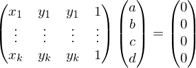

For a least-squares solution, we compute


with

If we shift all points into the center of gravity, this becomes

Since is constant, we can focus on the upper left
  block
block  of
of  .
.
Find:

such that .
.
Find smallest eigenvalue of . Scale corresponding eigenvector to
  .
.
Consistent Normal Orientation
Construct minimal spanning tree between all points with an edge weight

where controls how points are penalized for being further away from each other, and
  controls how points are penalized for having non-parallel normal directions.
Start at one point where the normal direction is known, e.g. the point with the lowest coordinate. From there, walk over the spanning tree and flip normals to make them consistent.
Signed Distance Field Estimation
Impose a voxel grid on the input points. For each grid vertex, estimate the value of a signed distance function for the object.
For every voxel, consider some neighboring samples and compute a weighted average of the distance of the voxel center to the respective tangent planes:

Iso-Surface Extraction
Using Marching Cubes. Output is a watertight two-manifold mesh.
- Estimate tangent planes from point cloud
- Consistently orient normals
- Construct signed distance field from point / normal samples
- Extract iso-surface mesh
Tangent Plane Estimation
Given a local cloud of points
 , we want to find a least-squares regression plane
or, for more points:


For a least-squares solution, we compute


with

If we shift all points into the center of gravity, this becomes

Since
 is constant, we can focus on the upper left
  block
block  of
of  .
.Find:

such that
 .
.Find smallest eigenvalue of
 . Scale corresponding eigenvector to
  .
.Consistent Normal Orientation
Construct minimal spanning tree between all points with an edge weight

where
 controls how points are penalized for being further away from each other, and
  controls how points are penalized for having non-parallel normal directions.
Start at one point where the normal direction is known, e.g. the point with the lowest
 coordinate. From there, walk over the spanning tree and flip normals to make them consistent.
Signed Distance Field Estimation
Impose a voxel grid on the input points. For each grid vertex, estimate the value of a signed distance function for the object.
For every voxel, consider some neighboring samples and compute a weighted average of the distance of the voxel center
 to the respective tangent planes:
Iso-Surface Extraction
Using Marching Cubes. Output is a watertight two-manifold mesh.
Explain parametrization using Least Squares Conformal Maps!
A parametrization is called conformal iff it is angle-preserving:

 is conformal iff
or

or
 is orthogonal:

Furthermore, it is conformal iff its inverse
  is conformal.
 conformal
 conformal
 orthogonal
 orthogonal

Solve least squares problem

for parameters . In order to get a unique solution, fix at least two points.
Computing Discrete Gradients
Computing

over a triangle given by corner vertices

and parameter values .
.
For a point inside the triangle, the interpolated value of
  is
is


Geometrical derivation of : Consider the triangle edge
  . Along
  ,
,  does not change. Along the direction
  ,
,  changes most. The magnitude of the change is
  , where
  is the height of
  on
on  . Thus,

We can compute the height from the triangle area and base length:


Plugging this result back in gives

With this result, we get


 is conformal iff
or

or
 is orthogonal:
Furthermore, it
 is conformal iff its inverse
  is conformal.
 conformal
 conformal
 orthogonal
 orthogonal
Solve least squares problem

for parameters
 . In order to get a unique solution, fix at least two points.
Computing Discrete Gradients
Computing

over a triangle given by corner vertices

and parameter values
 .
.For a point
 inside the triangle, the interpolated value of
  is
is


Geometrical derivation of
 : Consider the triangle edge
  . Along
  ,
,  does not change. Along the direction
  ,
,  changes most. The magnitude of the change is
  , where
  is the height of
  on
on  . Thus,
We can compute the height
 from the triangle area and base length:

Plugging this result back in gives

With this result, we get


How to create a Globally Smooth Parametrization?
Idea: Split input mesh into multiple (approximately quadratic) patches. Compute a discrete harmonic parametrization for each one. Some vertices will have neighbors which lie in another patch. The requirement for harmonic parametrization

must take this into account.
Introduce transition functions which represent the transformation between patches
  and
and  .
.
 transforms the parameter
  which is given in the local coordinates of patch
  into the local coordinate system of patch
  .
.
Obviously, and
and 
Thus, the harmonic parametrization system becomes:

Problem: For vertices close to patch corners, the transformation used to map neighbors to the local coordinate system might be ambiguous.
Solution: Fix parameters of corner vertices to the patch corners. Let the remaining vertices relax.

must take this into account.
Introduce transition functions
 which represent the transformation between patches
  and
and  .
. transforms the parameter
  which is given in the local coordinates of patch
  into the local coordinate system of patch
  .
.Obviously,
 and
and 
Thus, the harmonic parametrization system becomes:

Problem: For vertices close to patch corners, the transformation used to map neighbors to the local coordinate system might be ambiguous.
Solution: Fix parameters of corner vertices to the patch corners. Let the remaining vertices relax.
What are the properties of a Delaunay triangulation?
The Delaunay triangulation maximizes the smallest interior angle.
The Delaunay triangulation of a point set is unique (unless a triangle circumcircle intersects more than 3 vertices).
Dual properties of Delaunay triangulations and Voronoi diagrams
The Delaunay triangulation of a point set is unique (unless a triangle circumcircle intersects more than 3 vertices).
Dual properties of Delaunay triangulations and Voronoi diagrams
| Delauny triangulation | Voronoi diagram |
| Each triangle circumcircle contains no other vertices in its interior. | Around each Voronoi vertex, there exists a smallest circumcircle touching at least 3 Voronoi sites and containing no sites in its interior. |
| For every edge, there exists an empty circle containing both endpoints. | For every Voronoi edge, there exists a circle containing both adjacent Voronoi sites but no other sites. |
Give two definitions of the Voronoi diagram of a point set!
Given: Set of sites 
Closest Points
The Voronoi cell of a site
  is given by the set of all points which are closer to
  than to any other site
  :
:

Halfspace Intersection
Each pair of sites divides the space into a halfspace points which are closer to
  than to

Then, can be described as the intersection of all halfspaces formed with other sites:

From this definition, it is obvious that all Voronoi cells are convex.

Closest Points
The Voronoi cell
 of a site
  is given by the set of all points which are closer to
  than to any other site
  :
:
Halfspace Intersection
Each pair of sites
 divides the space into a halfspace points which are closer to
  than to

Then,
 can be described as the intersection of all halfspaces formed with other sites:
From this definition, it is obvious that all Voronoi cells are convex.
How to compute a Discrete Harmonic Parametrization? Give three examples for weights!
Given a mesh with disk topology of points  in the mesh domain
  , find points
  in the parameter domain
  .
.
A function is harmonic if its Laplace is zero, i.e.

Use a spring model: Edges of the mesh are mapped to springs. Fix parameters of mesh boundary points. Relax remaining points to equilibrium by solving

i.e.

Solve two linear systems:


To satisfy Tutte's theorem (and thus ensure a valid parametrization), use a concave boundary shape (circle, square) and have only positive spring weights.
Uniform Weights

Distributes vertices regularly in the parameter domain. No mesh structure is considered. Strong length and angular distortion.
Chordal Weights

Considers vertex distances. Low length distortion, but angular distortion is not controlled and thus high.
Cotangent Weights

In practice, low length and angular distortion. However, can lead to negative weights (violating Tutte's theorem).
 in the mesh domain
  , find points
  in the parameter domain
  .
.A function
 is harmonic if its Laplace is zero, i.e.
Use a spring model: Edges of the mesh are mapped to springs. Fix parameters of mesh boundary points. Relax remaining points to equilibrium by solving

i.e.

Solve two linear systems:


To satisfy Tutte's theorem (and thus ensure a valid parametrization), use a concave boundary shape (circle, square) and have only positive spring weights.
Uniform Weights

Distributes vertices regularly in the parameter domain. No mesh structure is considered. Strong length and angular distortion.
Chordal Weights

Considers vertex distances. Low length distortion, but angular distortion is not controlled and thus high.
Cotangent Weights

In practice, low length and angular distortion. However, can lead to negative weights (violating Tutte's theorem).
How can you estimate the distortion introduced by a parametrization?
Given a parametrization

consider the Jacobian of at some point
  :
:

and its Singular Value Decomposition

 and
and  are orthonormal, i.e. rotation matrices.
  is a diagonal matrix and corresponds to an axis-aligned scaling.
  thus can be interpreted as a concatenation of a rotation, a scaling and again a rotation. The distortion at
  can thus be inferred from
  and
and  :
:

consider the Jacobian of
 at some point
  :
:
and its Singular Value Decomposition

 and
and  are orthonormal, i.e. rotation matrices.
  is a diagonal matrix and corresponds to an axis-aligned scaling.
  thus can be interpreted as a concatenation of a rotation, a scaling and again a rotation. The distortion at
  can thus be inferred from
  and
and  :
:- Conformal / angle preserving:

- Area preserving:

- Isometry:

Explain Stretch Minimizing Parametrization!
Discrete Harmonic Parametrization may introduce unwanted stretch.
Idea: Repeat: Compute Harmonic Parametrization. Compute local stretch measures. Update weights according to local stretch measures.
Stretch Measure
SVD of Jacobian of

Stretch Measure:

 : Ellipsoid in
  is enlarged by
  . In order to make it smaller, push parameter positions away from each other in
  . To achieve this, decrease local spring weights.
 : Ellipsoid in
  is shrunk by
  . In order to make it bigger, pull parameter positions closer together in
  . To achieve this, increase local spring weights.
This gives the update rule:

Idea: Repeat: Compute Harmonic Parametrization. Compute local stretch measures. Update weights
 according to local stretch measures.
Stretch Measure
SVD of Jacobian of


Stretch Measure:

 : Ellipsoid in
  is enlarged by
  . In order to make it smaller, push parameter positions away from each other in
  . To achieve this, decrease local spring weights.
 : Ellipsoid in
  is shrunk by
  . In order to make it bigger, pull parameter positions closer together in
  . To achieve this, increase local spring weights.
This gives the update rule:

What is Light Tracing? What is Instant Radiosity?
Light Tracing
Reverse Monte Carlo Path Tracing. Start pathes in random light sources. In the absorption case, connect from the current point to the viewer. Advantage: Can detect high energy pathes.
Instant Radiosity
Efficient diffuse illumination utilizing Light Tracing and hardware rasterization.
Shoot photons from light sources. At every bounce, place a point light source at the photon position and render the scene with diffuse lighting and shadow mapping. Accumulate the brightness values of all pixels in a buffer (weighted by current photon energy).
Corresponds to bi-directional evaluation of pathes:

Explain the photon path notation! Give expressions for Phong Lighting, Ray Tracing, Radiosity, Path Tracing and Photon Mapping!
-
 absorption in the eye
 -
 diffuse reflection
 -
 glossy reflection
 -
 specular reflection
 -
 emission from a light source
Phong Lighting

One surface interaction. Diffuse or glossy.
Ray Tracing

Tracing from the eye. Arbitrary many specular reflections, then one final Phong lighting step.
Radiosity

Only diffuse reflections.
Path Tracing

A series of arbitrary reflections. Then, one final phong lighting step to connect to light source.
Photon Mapping

Arbitrary photon pathes.
Explain Photon Mapping!
Photon Generation
Shoot photons from all light sources:
Point light: Identical position. Uniform spherical distribution of directions.
Directional light: Identical direction. Uniform distribution of positions.
Area light: Uniform distribution of positions on the surface. Cos-thetha weighted distribution of directions.
For multiple light sources with different intensities: Adjust photon energy or photon frequency.
Optimization: Use projection maps to only shoot photons into directions where geometry is. Also requires scaling of energy:

Photon Tracing
On interaction with a surface with diffuse and specular reflection coefficients ,
,  :
:
Russian Roulette: Generate random number
Information stored in the photon map:
 : position
 : photon power (flux per solid angle)
 : angle of incidence
Radiance Estimate
Replace the recursive term in the Rendering Equation with a radiance estimate from the photon map. For a point , find the
  nearest neighbor samples from the photon map and compute


where

Rendering
Decompose the Rendering Equation


Evaluate the following factorizations:
Shoot photons from all light sources:
Point light: Identical position. Uniform spherical distribution of directions.
Directional light: Identical direction. Uniform distribution of positions.
Area light: Uniform distribution of positions on the surface. Cos-thetha weighted distribution of directions.
For multiple light sources with different intensities: Adjust photon energy or photon frequency.
Optimization: Use projection maps to only shoot photons into directions where geometry is. Also requires scaling of energy:

Photon Tracing
On interaction with a surface with diffuse and specular reflection coefficients
 ,
,  :
:Russian Roulette: Generate random number

-
 : Diffuse reflection. Store in photon map. Continue tracing (TODO: Which direction?).
 -
 : Specular reflection. Continue tracing (TODO: Which direction?).
 -
 : Absorption. Store in photon map.
Information stored in the photon map:

 : position
 : photon power (flux per solid angle)
 : angle of incidence
Radiance Estimate
Replace the recursive term in the Rendering Equation with a radiance estimate from the photon map. For a point
 , find the
  nearest neighbor samples from the photon map and compute

where

Rendering
Decompose the Rendering Equation


-
 : Diffuse reflections. Direction independent.
 -
 : Specular reflections.
 -
 : Direct illumination.
 -
 : Diffuse illumination.
 -
 : Caustic illumination.
Evaluate the following factorizations:
-
 Direct Illumination. Compute using ray casting / hemisphere sampling.
 -
 Specular / Glossy Reflections. Compute using MCPT.
 -
 Radiosity. Compute using radiance estimate from diffuse photon map.
 -
 Caustics. Compute using radiance estimate from caustic photon map.
How is the Photon Map stored? How are k-nearest-neighbor queries performed?
kD-Tree
Store photons in a balanced kD-Tree (i.e., a binary tree) with entries . The two child nodes of an inner node
  are
are  and
and  .
.
A balanced kD-Tree is constructed by successive median splits.
kD-Tree k-NN Search
Input:
 : query point
 : root node of subtree to be searched
Global variables:
 : priority queue containing k-best search results
 : distance from
  to furthest result in
  , or
, or  if less than
  results
knn( ,
,  ):
):
if( is a leaf)
insert into
into 
update
else
if is left of split plane
knn( ,
,  )
)
if distance to split plane
knn( ,
,  )
)
else
knn( ,
,  )
)
if distance to split plane
knn( ,
,  )
)
More efficient: Compare squared distances
Store photons in a balanced kD-Tree (i.e., a binary tree) with entries
 . The two child nodes of an inner node
  are
are  and
and  .
.A balanced kD-Tree is constructed by successive median splits.
kD-Tree k-NN Search
Input:
 : query point
 : root node of subtree to be searched
Global variables:
 : priority queue containing k-best search results
 : distance from
  to furthest result in
  , or
, or  if less than
  results
knn(
 ,
,  ):
):if(
 is a leaf)
insert
 into
into 
update

else
if
 is left of split plane
knn(
 ,
,  )
)if distance to split plane

knn(
 ,
,  )
)else
knn(
 ,
,  )
)if distance to split plane

knn(
 ,
,  )
)More efficient: Compare squared distances
Why is Hierarchical Radiosity more efficient than simple Shooting / Gathering?
Adaptive Refinement
Only refines patches whose form factors are large, thus generates fewer patches than uniform refinement.
Generate fewer links
For each element, there is only a constant number of other elements for which the form factor is large. All other elements are connected on different hierarchy levels. Thus, the number of links generated by Hierarchical Radiosity is linear in the number of elements while for classical Radiosity it is quadratic.
Name three ways to estimate Form Factors for Radiosity computation!
Sampling
Monte Carlo Sampling: Generate random points according to a distribution
  and evaluate

Nusselt Analogon
Given sender patch with area .
.
Project sender patch onto hemisphere of receiving patch:

where is the angle between sending patch normal and projection direction and
  is the distance between the two patches.
Project result into plane:


The form factor is the covered portion of the unit circle.


Problem: Assumptions only hold for patches that are sufficiently far away.
Hemicube
Rasterize 5 sides of a hemicube placed around a point on .
.
Denote by the set of pixels that see patch
  . Then,

where are pre-calculated form factors for the individual pixels of the hemicube.
Monte Carlo Sampling: Generate random points
 according to a distribution
  and evaluate
Nusselt Analogon
Given sender patch with area
 .
.Project sender patch onto hemisphere of receiving patch:

where
 is the angle between sending patch normal and projection direction and
  is the distance between the two patches.
Project result into plane:


The form factor is the covered portion of the unit circle.


Problem: Assumptions only hold for patches that are sufficiently far away.
Hemicube
Rasterize 5 sides of a hemicube placed around a point on
 .
.Denote by
 the set of pixels that see patch
  . Then,
where
 are pre-calculated form factors for the individual pixels of the hemicube.
Explain Monte Carlo Path Tracing!
MCPT solves the Rendering Equation using Monte Carlo Integration. The space over which is integrated is the space of all photon paths. Relevant paths are only those which carry energy: Starting from the eye and ending in an emissive surface:

The radiance at the end of this path is
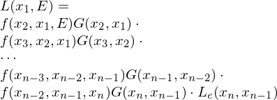
(for every photon bounce, there is one term )
)
MCPT():
for each pixel

for


 :
:

if
(emit)
return
else
(reflect)
generate random direction over
over 
return
If we choose

the return statement in the reflect case simplifies to just


The radiance at the end of this path is

(for every photon bounce, there is one term
 )
)MCPT():
for each pixel

for


 :
:
if

(emit)
return

else
(reflect)
generate random direction
 over
over 
return

If we choose

the return statement in the reflect case simplifies to just

What are two possible extensions for Monte Carlo Path Tracing?
Direct Lighting
Force all paths to end in a light source: When a photon would normally die, compute the direct illumination at its current position.
Sub-Paths
At each bounce, add one path that ends there. Needs to count total number of pathes generated.
Force all paths to end in a light source: When a photon would normally die, compute the direct illumination at its current position.
Sub-Paths
At each bounce, add one path that ends there. Needs to count total number of pathes generated.
What is the difference between Global Illumination algorithms and Image-Based Rendering?
Global Illumination
Simulation of light based on a physical model and a geometric representation of a scene.
Image-Based Rendering
Interpolation of collected data to synthesize an of a new viewpoint. Often with few / no scene geometry.
Simulation of light based on a physical model and a geometric representation of a scene.
Image-Based Rendering
Interpolation of collected data to synthesize an of a new viewpoint. Often with few / no scene geometry.
Name the two ways to think about light in physics? What effects can be explained by which model? Which model is used for Global Illumination algorithms?
Waves
Interference
Diffraction
Polarization
Particle / Photon
Reflection
Refraction
Scattering
Photon model realizes more important effects and is thus used in Global Illumination
Interference
Diffraction
Polarization
Particle / Photon
Reflection
Refraction
Scattering
Photon model realizes more important effects and is thus used in Global Illumination
Give the Rendering Equation in both formulations and explain all its terms!
Hemisphere Formulation

 : Incoming radiance at point
  from direction
 : Emitted radiance
 : Hemisphere over the surface at point
 : Intersection point of ray starting at
  with direction
  with the scene
 : BRDF: portion of light which enters from direction
  at
at  that is reflected into direction
 : Angle between
  and the normal vector of the surface at
Surface Formulation

where

and


 : Incoming radiance at point
  from direction
 : Emitted radiance
 : Hemisphere over the surface at point
 : Intersection point of ray starting at
  with direction
  with the scene
 : BRDF: portion of light which enters from direction
  at
at  that is reflected into direction
 : Angle between
  and the normal vector of the surface at
Surface Formulation

where

and

What simplifications are made for Radiosity? Derive the Radiosity Equation!
Simplification 1: Assume only diffuse surfaces.
Instead of BRDF , use reflectance
  .
.
Instead of radiances , use radiosity
  .
.
Resulting Radiosity Equation:


Simplification 2: Spatial Discretization
Assume scene consisting of patches with constant radiosity

Plug the Radiosity Equation into this:


We know that is constant over
  (with value
  ), thus we can pull it out of the integral:


with the Form Factors

Instead of BRDF
 , use reflectance
  .
.Instead of radiances
 , use radiosity
  .
.Resulting Radiosity Equation:


Simplification 2: Spatial Discretization
Assume scene consisting of patches
 with constant radiosity
Plug the Radiosity Equation into this:


We know that
 is constant over
  (with value
  ), thus we can pull it out of the integral:


with the Form Factors

Write the Radiosity Equation as a linear system and explain two ways to evaluate it! Which approach is better?
Linear Radiosity System

where
 are radiosity values
 is emitted radiosity
 is a diagonal matrix of reflectance values
 is the form factor matrix
Rearrange:


Expand using von-Neumann series


Gathering


Product requires row-wise evaluation of all form factors in
  (
( complexity)
Shooting
Idea: Only transport distribute energy from patches with high radiosity. Evaluate one colum of at a time.
Store a tuple for each patch:
 : accumulated radiosity on patch
 : unshot radiosity on patch
Repeat:
More efficient than Gathering but still complexity.

where
 are radiosity values
 is emitted radiosity
 is a diagonal matrix of reflectance values
 is the form factor matrix
Rearrange:


Expand using von-Neumann series


Gathering


Product
 requires row-wise evaluation of all form factors in
  (
( complexity)
Shooting
Idea: Only transport distribute energy from patches with high radiosity. Evaluate one colum of
 at a time.
Store a tuple
 for each patch:
 : accumulated radiosity on patch
 : unshot radiosity on patch
Repeat:
- Pick patch
 with highest unshot radiosity
- Update all other patches
 :
: -


More efficient than Gathering but still
 complexity.
Define the Form Factors for Radiosity! When are the form factors large / small? How are reciprocal form factors related? Give the Flux Equation!


First integral: Averaging over receiver
 . Second integral: Accumulating over sender
  .
. describes how much influence the radiosity of patch
  has on the radiosity of patch
  .
. small,
  large:
  high.
high. large,
  small:
  low.
low.Reciprocal Form Factors


Flux Equation
Flux is radiosity times area:


Radiosity is flux per area:


Explain Hierarchical Radiosity!
Radiosity is very smooth across most patches. Use adaptive refinement to only subdivide where form factors change. Problem: Subdivision leads to  complexity since each patch can interact with each other one.
Solution: Allow interactions across subdivision levels.
Adaptive Refinement
Idea: where form factors are large, subdivide the larger patch
refine( ,
,  ):
):
if ( &&
&&  )
)
link( ,
,  )
)
else if ( )
)
if (subdivide( ) >
) >  )
)
refine( ,
,  )
)
refine( ,
,  )
)
refine( ,
,  )
)
refine( ,
,  )
)
else
link( ,
,  )
)
else
if (subdivide( ) >
) >  )
)
refine( ,
,  )
)
refine( ,
,  )
)
refine( ,
,  )
)
refine( ,
,  )
)
else
link( ,
,  )
)
Solution
Alternatingly, apply to all unsubdivided patches
Gather
gather( ):
):
 .in
.in 
for (all links )
)
 .in
.in 
 .in +
.in +  .out
.out
gather( )
)
gather( )
)
gather( )
)
gather( )
)
Push-Pull
pushpull( )
)
if ( has children)
push
 in
in 
 in
in  .in
.in
 in
in 
 in
in  .in
.in
 in
in 
 in
in  .in
.in
 in
in 
 in
in  .in
.in
recurse
pushpull( )
)
pushpull( )
)
pushpull( )
)
pushpull( )
)
pull

else
convert incoming to outgoing radiance
 in
in
 complexity since each patch can interact with each other one.
Solution: Allow interactions across subdivision levels.
Adaptive Refinement
Idea: where form factors are large, subdivide the larger patch
refine(
 ,
,  ):
):if (
 &&
&&  )
)link(
 ,
,  )
)else if (
 )
)if (subdivide(
 ) >
) >  )
)refine(
 ,
,  )
)refine(
 ,
,  )
)refine(
 ,
,  )
)refine(
 ,
,  )
)else
link(
 ,
,  )
)else
if (subdivide(
 ) >
) >  )
)refine(
 ,
,  )
)refine(
 ,
,  )
)refine(
 ,
,  )
)refine(
 ,
,  )
)else
link(
 ,
,  )
)Solution
Alternatingly, apply to all unsubdivided patches
- Gathering Step
- Push-Pull Step
Gather
gather(
 ):
): .in
.in 
for (all links
 )
) .in
.in 
 .in +
.in +  .out
.outgather(
 )
)gather(
 )
)gather(
 )
)gather(
 )
)Push-Pull
pushpull(
 )
)if (
 has children)
push
 in
in 
 in
in  .in
.in in
in 
 in
in  .in
.in in
in 
 in
in  .in
.in in
in 
 in
in  .in
.inrecurse
pushpull(
 )
)pushpull(
 )
)pushpull(
 )
)pushpull(
 )
)pull

else
convert incoming to outgoing radiance
 in
inExplain the de Casteljau algorithm!
de Casteljau algorithm gives a geometric procedure to construct points on Bézier curves.
Example: Given control points (cubic spline), we compute


Note how this schema iteratively evaluates the Bernstein polynomials for all coefficients:


Useful properties:
Example: Given control points
 (cubic spline), we compute


Note how this schema iteratively evaluates the Bernstein polynomials for all coefficients:


Useful properties:
- Numerically robust: Sequence of affine combinations (instead of sum of scaled polynomial coefficients)
- First derivative:

What are spline curves? How are spline curves constructed from Bézier curves?
Spline curves: Piecewise polynomial curves which are maximally smooth:
Polynomial degree

 continuous
Constructing Spline curves
This allows to create a cubic spline curve by only specifying A-frame vertices:
Polynomial degree


 continuous
Constructing Spline curves
- Degree 1: Linear segments. Connect endpoints for
- Degree 2: Quadratic segments. Connect endpoints for
- Degree 3: Cubic segments. Connect endpoints for
 continuity.
 continuity.Use identical vector for first and last edge of subsequent segments for
  continuity.
 continuity.Use identical vector for first and last edge of subsequent segments for
  continuity.Extend the middle edges of both segments and find the intersection point: If the so-created A-frame splits each pair of collinear edges in a 1:1 ratio, the connection between the segments is
  continuous.
This allows to create a cubic spline curve by only specifying A-frame vertices:
- Connect A-frame vertices by edges and split 1:1:1
- Add edges between each first and last vertex between neighboring edges and split 1:1
- Connect each 4 vertices with one cubic spline
How to create Freeform Surfaces from Bézier curves?
Tensor Product Patches
given a grid of coefficients for
for  ,
,  , compute a surface
First, compute interpolated control points for parameter
  :
:

Then, compute the interpolated point along the curve of the generated control points for parameter
  :
:


tensor
given a grid of coefficients
 for
for  ,
,  , compute a surface
First, compute interpolated control points
 for parameter
  :
:
Then, compute the interpolated point along the curve of the generated control points
 for parameter
  :
:


tensor
How to compute an interpolating spline curve?
Exploit endpoint interpolation of spline segments. Compute positions for spline control points  such that the positions of spline endpoints match the desired interpolation positions
  .
.
Example: Cubic splines
Given spline control points , we can compute the position of the closest spline endpoint as

Set up a linear system
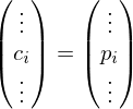
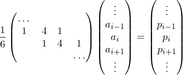
and solve for .
.
 such that the positions of spline endpoints match the desired interpolation positions
  .
.Example: Cubic splines
Given spline control points
 , we can compute the position of the closest spline endpoint as
Set up a linear system


and solve for
 .
.What types of culling are there?
Back-face culling
Skipping polygons which face away from the viewer (on back sides of objects)
View frustum culling
Skipping objects which are outside the region covered by the camera view frustum
(often used in conjunction with appropriate hierarchical optimization structures)
Portal culling
Only rendering objects which are visible inside a restricted region of the current view frustum, generated by the shape of a portal
1. render current room
2. for all portals of the current room inside the current frustum: narrow down the frustum and repeat step 1 in the room behind the respective portal
Occlusion culling
Skipping objects which are in the viewing frustum but hidden by other objects in front of it
Explain Shadow Mapping! What problem is solved by Perspective Shadow Mapping, and how?
Insight: Shadowing is a visibility problem like the one for rendering in general.
Problem: Discretization of off-screen depth buffer leads to aliasing artifacts. The size of one texel of the shadow map in the final camera image is given by the following approximation:

 : shadow map resolution
 : distance from light source to shadow surface (affects Perspective Aliasing)
 : angle between shadow surface and shadow map projection plane normal (affects Projective Aliasing)
 : angle between shadow surface and image plane normal (affects Projective Aliasing)
 : distance from shadow surface to camera (affects Perspective Aliasing)
 can be decreased at the cost of memory / computation
 can not be changed.
Goal: make as large as possible.
Solution: Apply the frustum transform of the camera to the scene before shadow map rendering and lookup. This effectively moves the camera center to infinity and thus minimizes the Perspective Aliasing caused by the camera distance.
- Render scene from the position of the light source into an off-screen depth buffer
- Render scene from the camera view. For every pixel: Compute position w.r.t. view from light source. Look up depth value from off-screen depth buffer. If
 , the pixel is in shadow.
Problem: Discretization of off-screen depth buffer leads to aliasing artifacts. The size of one texel of the shadow map in the final camera image is given by the following approximation:

 : shadow map resolution
 : distance from light source to shadow surface (affects Perspective Aliasing)
 : angle between shadow surface and shadow map projection plane normal (affects Projective Aliasing)
 : angle between shadow surface and image plane normal (affects Projective Aliasing)
 : distance from shadow surface to camera (affects Perspective Aliasing)
 can be decreased at the cost of memory / computation
 can not be changed.
Goal: make
 as large as possible.
Solution: Apply the frustum transform of the camera to the scene before shadow map rendering and lookup. This effectively moves the camera center to infinity and thus minimizes the Perspective Aliasing caused by the camera distance.
What are advantages and disadvantages of Shadow Maps and Shadow Volumes?
| Shadow Maps | Shadow Volumes |
| any shadow geometry | shadow geometry must be manifold poly-mesh |
| omni-directional lights require multiple shadow maps | omni-directional lights are no special case |
| requires additional resources (off-screen depth textures) | requires additional computation (projecting shadow volumes) |
| aliasing / depth bias artifacts | exact shadows |
What is a 2-manifold? How can you tell whether a triangle mesh is a 2-manifold?
Two-manifold: A surface where every local vicinity is homeomorphic to a disc.
Triangle mesh criteria for 2-manifoldness:
Triangle mesh criteria for 2-manifoldness:
- the interior of faces is flat and hence homeomorphic to a disc
- at every edge, there must be exactly 2 adjacent faces (except for boundary edges with 1 adjacent face)
- every vertex must have a uniquely defined 1-ring neighborhood
Give the Euler Formula and prove it!

Start with a closed mesh with genus 0: 1 vertex surrounded by 1 face:

Three fundamental operation for extending the mesh:
Add new vertex connected by one edge

Connect two existing vertices by a new edge

Genus change: Connect two holes (i.e. faces) by one new edge, thus merging the two holes into one

 increases by 1
Give the Euler Formula and derive the three Magic Numbers!

Magic Number: 2 times as many faces as vertices


Magic Number: Average vertex valence is 6


Magic Number: 5 platonic solids
A platonic solids with Schläfli symbol
 is a polygonal mesh fulfilling the following properties:
-

- All faces are
 -gons:
  (where
  )
) - All vertices have valence
 :
:  (where
  )
)


Number of edges cannot be negative:

Since
 and
and  :
:

Gives only 5 solutions for
 :
:-
 : Tetrahedron (4 triangular faces, self-dual)
 -
 : Octahedron (8 triangular faces, dual to Cube)
 -
 : Cube (6 square faces, dual to Octahedron)
 -
 : Icosahedron (20 triangular faces, dual to Dodecahedron)
 -
 : Dodecahedron (12 pentagonal faces, dual to Icosahedron)
How are 3D volumes be represented using quadrics? Give the quadrics for spheres, cylinders, cones! How are quadrics transformed? How to compute ray / quadric intersections?
Scalar function  . Inside < 0, surface = 0, outside > 0. All quadratic trivariate functions are given by

or

or

or

Sphere
at center with radius
  :
:


Cylinder
along the axis around
  with radius
  :
:


Cone
apex at , opening along the
  axis with an angle of


Quadric Transformation
Given a point on the surface of a quadric
  :
:

we apply a transformation to :
:

we obtain


Thus, the quadric after application of the transformation is:

Ray / Quadric Intersections


Has 0, 1, or 2 real solutions.
 . Inside < 0, surface = 0, outside > 0. All quadratic trivariate functions are given by
or

or

or

Sphere
at center
 with radius
  :
:


Cylinder
along the
 axis around
  with radius
  :
:


Cone
apex at
 , opening along the
  axis with an angle of


Quadric Transformation
Given a point
 on the surface of a quadric
  :
:
we apply a transformation to
 :
:
we obtain


Thus, the quadric after application of the transformation is:

Ray / Quadric Intersections


Has 0, 1, or 2 real solutions.
Explain Volume Ray Casting!
Volume Rendering Integral
Given functions for color and opacity
  (where 0 = transparent and
  = opaque), the color for a ray
  is given by


Discretization


 : opacity (0 = transparent,
  = opaque)
 : normalized transparency (0 = opaque, 1 = transparent)
 : normalized opacity (0 = transparent, 1 = opaque)

We only want opaque pixels to emit color:

Volume Rendering Integral
Given functions for color and opacity
  (where 0 = transparent and
  = opaque), the color for a ray
  is given by


Discretization


 : opacity (0 = transparent,
  = opaque)
 : normalized transparency (0 = opaque, 1 = transparent)
 : normalized opacity (0 = transparent, 1 = opaque)

We only want opaque pixels to emit color:

Back-to-Front Evaluation
Start:

Update:

Front-to-Back Evaluation
Start:


Update:


Early abort if
Given functions for color
 and opacity
  (where 0 = transparent and
  = opaque), the color for a ray
  is given by


Discretization


 : opacity (0 = transparent,
  = opaque)
 : normalized transparency (0 = opaque, 1 = transparent)
 : normalized opacity (0 = transparent, 1 = opaque)
We only want opaque pixels to emit color:

Volume Rendering Integral
Given functions for color
 and opacity
  (where 0 = transparent and
  = opaque), the color for a ray
  is given by


Discretization


 : opacity (0 = transparent,
  = opaque)
 : normalized transparency (0 = opaque, 1 = transparent)
 : normalized opacity (0 = transparent, 1 = opaque)
We only want opaque pixels to emit color:

Back-to-Front Evaluation
Start:

Update:

Front-to-Back Evaluation
Start:


Update:


Early abort if

Explain the Marching Cubes algorithm! What are its disadvantages?
Given: Volumetric representation 
Impose regular grid of cubes over the volume.
For every cube cell:
Disadvantages:

Impose regular grid of cubes over the volume.
For every cube cell:
- Sample the values of
 at the eight cube vertices
 - Based on a lookup table with
 entries, decide which geometry to generate for this cell
 - Compute intersection positions for vertices on the cube edges. For instance, the position of the vertex right of
 is
is

Disadvantages:
- Creates mesh which can be highly over-sampled (requires Decimation) and contain bad triangle shapes (requires Mesh Optimization / Re-Meshing)
- Linear interpolation of distance values approximates smooth surfaces: Sharp features within cells are lost
- Aliasing artifacts due to alignment of the voxel grid. Increasing voxel resolution only reduces the size of the artifacts but they never go away
Give the Bernstein polynomials! What are their properties?
Partition of unity:


Define the Bernstein polynomial

Bezier curve

Properties


Define the Bernstein polynomial

Bezier curve

Properties
- Partition of unity
- Non-negativity
- Maximum
- Endpoint interpolation
- Symmetry
- Recursion
 (by definition)Because of this, the affine combination of coefficients is geometrically meaningful.
 for
for  Points of the curve are actually convex combinations of the coefficients. Thus, the curve will lie inside the convex hull of the control points.
 has its maximum at
  This ensures local influence of the control points.
 , thus
 , thus

 where
where  and
and 
What problems are addressed by the Extended Marching Cubes algorithm? How does it solve them?
Problems of Marching Cubes
Solution: Directed Distances
instead of an iso-value, store three directed distances for every vertex: exact distance to the surface crossing along every cube edge
Solution: Feature Detection / Sampling / Reconstruction
Feature Detection
based on the gradient values at the edge intersections, compute normal vectors:

find the two normal vectors which span the largest angle


find the normal which forms the smallest angle to the orthogonal direction


If , we have detected a feature.
If additionally , the current feature is a corner feature (two large opening angles). Otherwise, it is an edge feature (one large opening angle).
Feature Sampling
Find intersection point of tangent planes:


This might not have a unique solution:
Over-determined: No common intersection point. Find least-squares solution (closest to all planes).
Under-determined: Infinitely many intersection points. Find least-norm solution (closest to voxel center).
Solve using SVD:


Feature Reconstruction
Look up cell configuration from Marching Cubes table. If in a feature cell, insert feature vertex at computed position and connect with a triangle fan. Flip edges so they align with feature edges.
- edge intersections are computed using linear interpolation (inaccurate)
- assumes smooth isosurface: sharp features within cells are lost (aliasing problem)
Solution: Directed Distances
instead of an iso-value, store three directed distances for every vertex: exact distance to the surface crossing along every cube edge
Solution: Feature Detection / Sampling / Reconstruction
Feature Detection
based on the gradient values at the edge intersections, compute normal vectors:

find the two normal vectors
 which span the largest angle

find the normal
 which forms the smallest angle to the orthogonal direction


If
 , we have detected a feature.
If additionally
 , the current feature is a corner feature (two large opening angles). Otherwise, it is an edge feature (one large opening angle).
Feature Sampling
Find intersection point of tangent planes:


This might not have a unique solution:
Over-determined: No common intersection point. Find least-squares solution (closest to all planes).
Under-determined: Infinitely many intersection points. Find least-norm solution (closest to voxel center).
Solve using SVD:


Feature Reconstruction
Look up cell configuration from Marching Cubes table. If in a feature cell, insert feature vertex at computed position and connect with a triangle fan. Flip edges so they align with feature edges.
Explain the Singular Value Decomposition!
Given  , a system

might be over- or under-determined. We still want to compute an approximate solution.
For any such , there exists the Singular Value Decomposition
 where
where
 is orthonormal:

 is orthonormal:
From this, we can construct the pseudo-inverse

where
where

Due to numerical imprecisions, we use

Now, we can compute a solution:


This solution is
 , a system
might be over- or under-determined. We still want to compute an approximate solution.
For any such
 , there exists the Singular Value Decomposition
 where
where is orthonormal:

 is orthonormal:
From this, we can construct the pseudo-inverse

where

where

Due to numerical imprecisions, we use

Now, we can compute a solution:


This solution is
- a solution in the least-squares sense if M is overdetermined
- a solution in the last-norm sense if M in underdetermined
Explain different ways to store meshes on disk and give the average amount of memory per vertex!
Face Set
For each triangle, store the position of all vertices.
 vertices
 triangles
 positions
 floats
 bytes
bytes
Shared Vertex
Store one list with positions of all vertices. For each triangle, store three indices into the vertex list.
For the vertex list:
 vertices
 positions
 floats
 bytes
bytes
For the triangles:
 vertices
 triangles
 indices (i.e. ints)
 bytes
bytes
Total
 bytes
bytes
Triangle Strips
Store a list of vertex positions. Each triple of vertices in that list defines one triangle. (Note: triangles have alternating winding)
 vertices
 triangles
 positions
 floats
 bytes
bytes
Representing general triangle meshes as triangle strips:
For each triangle, store the position of all vertices.
 vertices
 triangles
 positions
 floats
 bytes
bytesShared Vertex
Store one list with positions of all vertices. For each triangle, store three indices into the vertex list.
For the vertex list:
 vertices
 positions
 floats
 bytes
bytesFor the triangles:
 vertices
 triangles
 indices (i.e. ints)
 bytes
bytesTotal
 bytes
bytesTriangle Strips
Store a list of vertex positions. Each triple of vertices in that list defines one triangle. (Note: triangles have alternating winding)
 vertices
 triangles
 positions
 floats
 bytes
bytesRepresenting general triangle meshes as triangle strips:
- Apply 1:3-splits to allow for flexibility in mesh traversal.
- Generalized Triangle Strips: Store 1 additional bit per vertex, telling whether to replace the oldest or second-oldest vertex from the current triangle.
- Use multiple triangle strips for one mesh
Name and explain three mesh data structures for geometry processing!
Face Based
Store, for every face:
Problem: For arbitrary meshes, entries can be of different size (because of varying face valence)
Edge Based
Store, for every edge:
Advantage: Constant storage per entry
Problem: Start and end point are chosen arbitrarily. Traversal in both directions requires case distinctions.
Halfedge Based
Store, for every halfedge:
Advantage: Constant storage per entry, no directional ambiguity, can only represent manifold meshes
Enumerating 1-Ring Neighborhood
1. pick one outgoing halfedge from center vertex
2. do something with the current target vertex
3. go to the opposite halfedge
4. go to the next halfedge
5. if the current halfedge is not , go to 2
Store, for every face:
- pointers to all face vertices
- pointers to all adjacent faces
Problem: For arbitrary meshes, entries can be of different size (because of varying face valence)
Edge Based
Store, for every edge:
- 2 pointers to the edge endpoint vertices
- 2 pointers to the incident faces
- 4 pointers to adjacent edges (on each side, one in cw / ccw direction)
Advantage: Constant storage per entry
Problem: Start and end point are chosen arbitrarily. Traversal in both directions requires case distinctions.
Halfedge Based
Store, for every halfedge:
- pointer to target vertex
- pointer to incident face (to the left)
- pointer to next halfedge (leftmost outgoing halfedge from target vertex)
- pointer to opposite halfedge (not explicitly stored: store list of halfedge pairs. obtain pointer to opposite halfedge by flipping last bit of index)
- (sometime: previous halfedge)
Advantage: Constant storage per entry, no directional ambiguity, can only represent manifold meshes
Enumerating 1-Ring Neighborhood
1. pick one outgoing halfedge
 from center vertex
2. do something with the current target vertex
3. go to the opposite halfedge
4. go to the next halfedge
5. if the current halfedge is not
 , go to 2
Explain point based rendering techniques! In what cases are they used? How does real-time rendering work? What are disadvantages?
For very hi-res models, where triangle rendering would lead to multiple triangles mapping to the same pixel, it is more efficient to drop the triangle rendering and just render points.
Gaps between points filled by rendering splats (litte discs).
Possible improvements:
Real-time rendering of blended splat clouds: 2-Pass Rendering
Major disadvantage: For (approximately) correct visibility, point cloud needs to be rendered twice
Gaps between points filled by rendering splats (litte discs).
Possible improvements:
- Oriented Splats: Better approximation of object's silhouette (using normal information, e.g. from least-square plane of local neighborhood)
- Gouraud Splatting: Render blended blobs instead of discs (low-pass filter)
- Phong Splatting: Smoothly blend normal information, then shade in deferred rendering pass based on depth buffer and interpolated normals
Real-time rendering of blended splat clouds: 2-Pass Rendering
- render splat cloud to z-buffer only
- render colored and blended splat cloud again with depth write off and some depth bias
Major disadvantage: For (approximately) correct visibility, point cloud needs to be rendered twice
Explain how to transform geometry according to camera position and projection to the screen!
Concatenation of three matrices:

Look-at transform
Given a camera position , a desired viewing direction
  and an up vector
  , we compute a orthogonal coordinate system as follows:


Now, the matrix transforming points from camera space to world space is given by

The look-at transform is the inverse of this, transforming points from world space to local camera space:

Frustum transform
Transforms points from a frustum defined by the near / far plane distance of the camera and the extents of the near plane rectangle
  into the unit cube
  .
.  maps points on the near plane to
  and points on the far plane to
  .
.
Viewport transform
Transforms from the unit cube to pixel coordinates on a screen:


Look-at transform

Given a camera position
 , a desired viewing direction
  and an up vector
  , we compute a orthogonal coordinate system as follows:

Now, the matrix transforming points from camera space to world space is given by

The look-at transform is the inverse of this, transforming points from world space to local camera space:

Frustum transform

Transforms points from a frustum defined by the near / far plane distance of the camera
 and the extents of the near plane rectangle
  into the unit cube
  .
.  maps points on the near plane to
  and points on the far plane to
  .
.Viewport transform

Transforms from the unit cube to pixel coordinates on a
 screen:
What is trichromacity? What is metamerism?
Trichromacity
Cone cells in the eye only report one integral value, which is

where is the incoming color spectrum and
  is the response function of the given cone type. Since there are only three types of cone cells, each color stimulus can be described by a three-tuple
  , the tristimulus.
Metamerism
Due to trichromacity, different color spectra can map to the same tristimulus value and thus produce the same color impression.
Cone cells in the eye only report one integral value, which is

where
 is the incoming color spectrum and
  is the response function of the given cone type. Since there are only three types of cone cells, each color stimulus can be described by a three-tuple
  , the tristimulus.
Metamerism
Due to trichromacity, different color spectra can map to the same tristimulus value and thus produce the same color impression.
What is the CIE color model and why is it used?
Color system with artificial basis colors which allows all human visible colors to be represented by a triple of positive values.
This is not possible when using the natural red, green and blue base colors: In order to recreate the color impression of wavelengths between 450 and 550 nm, negative red light contributions would be necessary.
This is not possible when using the natural red, green and blue base colors: In order to recreate the color impression of wavelengths between 450 and 550 nm, negative red light contributions would be necessary.
Give transformation matrices for translation, scaling, shearing and rotation.
Translation
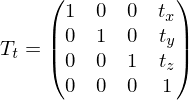
Scaling
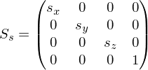
Shearing (here: x-axis is sheared into y direction)
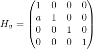
Rotation around x, y and z axis, respectively (counter-clockwise when rotation axis points towards observer, clockwise when looking into direction of the axis)
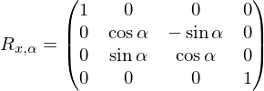
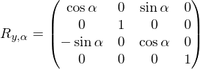
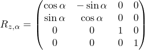

Scaling

Shearing (here: x-axis is sheared into y direction)

Rotation around x, y and z axis, respectively (counter-clockwise when rotation axis points towards observer, clockwise when looking into direction of the axis)


Give three basic projective transforms
Standard Projection
projects towards the origin onto plane
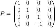
Central Point Projection
projects towards the origin onto a plane with normal at distance
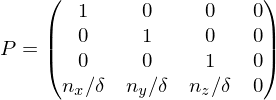
note: Standard Projection is a special case of this
Central Plane Projection
project onto plane through origin given by normal vector towards point
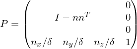
Degenerates to orthogonal projection for
projects towards the origin onto plane


Central Point Projection
projects towards the origin onto a plane with normal
 at distance

note: Standard Projection is a special case of this
Central Plane Projection
project onto plane through origin given by normal vector
 towards point

Degenerates to orthogonal projection for

Characterize linear, affine and projective transforms!
Linear Maps
A map which is
additive:
homogenous:
Representable by a transformation matrix :
:

Linear map preserve the origin.
Affine Maps
A map which is
composed of a linear map and a translation:

Affine transformations can be represented as a matrix-vector product by using extended coordinates:

Affine maps preserve collinearity of points and distance ratios.
Projective Maps
Represented by a matrix-vector product using homogeneous coordinates.
Projective maps preserve cross ratios:

A map
 which is
additive:

homogenous:

Representable by a transformation matrix
 :
:
Linear map preserve the origin.
Affine Maps
A map
 which is
composed of a linear map
 and a translation:
Affine transformations can be represented as a matrix-vector product by using extended coordinates:

Affine maps preserve collinearity of points and distance ratios.
Projective Maps
Represented by a matrix-vector product using homogeneous coordinates.
Projective maps preserve cross ratios:

How to construct the vanishing point of a line? (analytically and on paper)
A point and a direction


define the line

The standard projection of a point
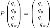
results, after de-homogenization, in the point

on the image plane.
Thus,

Let us only examine the x-coordinate of this and rearrange some terms:


Now, if and
and  ,
,


define the line

The standard projection of a point


results, after de-homogenization, in the point

on the image plane.
Thus,

Let us only examine the x-coordinate of this and rearrange some terms:


Now, if
 and
and  ,
,
How can 2D / 3D geometric objects be represented?
parametric: Range of a (uni- / multivariate) function mapping parameters to points on the object. Easy to produce points belonging to an object.
implicit: Function telling for each point in space whether it belongs to the object or not. Easy to test points for membership.
implicit: Function telling for each point in space whether it belongs to the object or not. Easy to test points for membership.
How are lines represented in parametric / implicit form?
Parametric
With base point , direction
  :
:

Implicit 2D
Find normal vector to
to  . Then, the line is given by all points
  for which
 .
.
Implicit 3D
Find two vectors orthogonal to
  . Then, the line is given by the intersection of the two planes given by
  , i.e. all points
  for which
 .
.
With base point
 , direction
  :
:
Implicit 2D
Find normal vector
 to
to  . Then, the line is given by all points
  for which
 .
.Implicit 3D
Find two vectors
 orthogonal to
  . Then, the line is given by the intersection of the two planes given by
  , i.e. all points
  for which
 .
.Explain Barycentric Coordinates and give a geometric interpretation!
Three non-collinear points  span a plane. Any point
  in this plane is given by an affine combination
 , where
or

The values are called the barycentric coordinates of
  .
.
 lies on the intersection of
an -iso-line which is parallel to
  ,
,
a -iso-line which is parallel to
  ,
,
a -iso-line which is parallel to
  .
.
 span a plane. Any point
  in this plane is given by an affine combination
 , where
or

The values
 are called the barycentric coordinates of
  .
. lies on the intersection of
an
 -iso-line which is parallel to
  ,
,a
 -iso-line which is parallel to
  ,
,a
 -iso-line which is parallel to
  .
.Give the steps of the Rendering Pipeline!
Input: 3D Geometry
Output: Image
In hardware: Transformation / Projection programmable in Vertex Shader. Lighting / Texturing programmable in Fragment Shader. Visibility Test may be done after / during Rasterization (Early-Z).
- Transformation / Projection
- Clipping
- Rasterization
- (Local) Lighting
- Texturing
- Visibility Test
Output: Image
In hardware: Transformation / Projection programmable in Vertex Shader. Lighting / Texturing programmable in Fragment Shader. Visibility Test may be done after / during Rasterization (Early-Z).
Explain the Bresenham / Midpoint algorithm for line drawing!
A line with integer-valued endpoints  should be rasterized. W.l.o.g., we assume
  and
and  (we can rotate / flip our pixel grid to fulfill these conditions).
The line is rasterized by starting with a point on the line at
  , and successively shifting
  to the right
 ,
,
or to the top right
 .
.
This decision is made based on whether the line passes above or below the midpoint

between and
and  .
.
This condition can be checked by deriving an implicit representation of the line . By taking
  , we can define a normal to
  as
as

and thus derive the implicit representation
 .
.
In order to decide whether to go East or Northeast, we introduce a decision variable, which is initially
 .
.
If , we go East:
Update .
.
Update .
.
If , we go Northeast:
Update .
.
Update .
.
Values for can be doubled, thus using only integer arithmetic.
 should be rasterized. W.l.o.g., we assume
  and
and  (we can rotate / flip our pixel grid to fulfill these conditions).
The line is rasterized by starting with a point
 on the line at
  , and successively shifting
  to the right
 ,
,or to the top right
 .
.This decision is made based on whether the line passes above or below the midpoint

between
 and
and  .
. This condition can be checked by deriving an implicit representation of the line
 . By taking
  , we can define a normal to
  as
as
and thus derive the implicit representation
 .
.In order to decide whether to go East or Northeast, we introduce a decision variable, which is initially
 .
.If
 , we go East:
Update
 .
.Update
 .
.If
 , we go Northeast:
Update
 .
.Update
 .
.Values for
 can be doubled, thus using only integer arithmetic.
Draw a unit cube using 1-Point / 2-Point / 3-Point Perspective!
1-Point:
Vanishing point is identical with the projection center
  . Draw lines from cube edge
  to
to  . The vanishing points of the cube diagonals
  are found by adding lines with distance
  to the projection center, parallel to the edges of the cube.
2-Point:
Vanishing points ,
,  lie on a line with the projection center
  . Given a cube edge
  , add connections from the end vertices to the vanishing points.
Now, consider shifting the upper corner of the cube into the projection center. Then,
  forms a right triangle with
  and
and  , where
  is the footpoint of
  . Given the lengths
  ,
,  , we can construct the vanishing points of the diagonals of the cube.
 and
and  can be found geometrically by constructing a half circle above
  and intersecting it with the perpendicular above
  .
.
3-Point:
Only the three vanishing points are given. The projection center
  is found by intersecting the three heights of the triangle
  . Based on these heights, we again use Thales' theorem to find the right triangles above the edges of the vanishing point triangle. By intersecting the angle bisectors with the respective edges, the diagonal vanishing points
  are found.
Vanishing point
 is identical with the projection center
  . Draw lines from cube edge
  to
to  . The vanishing points of the cube diagonals
  are found by adding lines with distance
  to the projection center, parallel to the edges of the cube.
2-Point:
Vanishing points
 ,
,  lie on a line with the projection center
  . Given a cube edge
  , add connections from the end vertices to the vanishing points.
Now, consider shifting the upper corner
 of the cube into the projection center. Then,
  forms a right triangle with
  and
and  , where
  is the footpoint of
  . Given the lengths
  ,
,  , we can construct the vanishing points of the diagonals of the cube.
 and
and  can be found geometrically by constructing a half circle above
  and intersecting it with the perpendicular above
  .
.3-Point:
Only the three vanishing points
 are given. The projection center
  is found by intersecting the three heights of the triangle
  . Based on these heights, we again use Thales' theorem to find the right triangles above the edges of the vanishing point triangle. By intersecting the angle bisectors with the respective edges, the diagonal vanishing points
  are found.
Flashcard set info:
Author: janisborn
Main topic: Informatik
Topic: Computergrafik
School / Univ.: RWTH Aachen
City: Aachen
Published: 18.05.2022
Card tags:
All cards (116)
no tags


 and
and 


 with uniform weights (does both normal and tangential smoothing).
 with cotangent weights (does mostly normal smoothing).
 distributed according to


 , the smaller the variance of the quotient
 ,
, until
until  . Then, return


 until
until  .
.


 -dimensional integral.


 where
where if
if  if
if  if
if 


